This section will show you how to build a recommendation model using item descriptions and user purchases. The model combines item-based collaborative filtering with some information about the items. We will include the item description using a monolithic hybrid system with feature combination. The recommender will learn from the two data sources in two separate stages.

Following the approach described in Chapter 3, Recommender Systems, let's split the data into the training and the test set:

which_train <- sample(x = c(TRUE, FALSE),size = nrow(ratings_matrix),replace = TRUE,prob = c(0.8, 0.2))recc_data_train <- ratings_matrix[which_train, ]
recc_data_test <- ratings_matrix[!which_train, ]

Now, we can build an IBCF model using Recommender. Since the rating matrix is binary, we will set the distance method to Jaccard. For more details, look at the Collaborative filtering on binary data section in Chapter 3, Recommender Systems. The remaining parameters are left to their defaults:

recc_model <- Recommender(data = recc_data_train,method = "IBCF",parameter = list(method = "Jaccard"))

The engine of IBCF is based on a similarity matrix about the items. The distances are computed from the purchases. The more the number of items purchased by the same users, the more similar they are.

We can extract the matrix from the sim element in the slot model. Let's take a look at it:

class(recc_model@model$sim)
## dgCMatrix
dim(recc_model@model$sim)
## _166_ and _166_

The matrix belongs to the dgCMatrix class, and it is square. We can visualize it using image:

image(recc_model@model$sim)

The following image is the output of the preceding code:

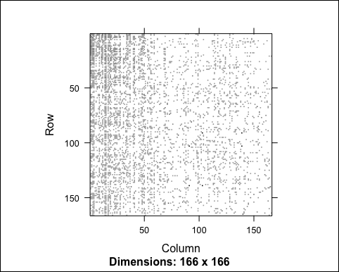
We can't identify any clear pattern, and it's because the items are not sorted. Let's take a look at the range of values:

range(recc_model@model$sim)
## _0_ and _1_

All the distances are between 0 and 1.

Our target is to combine the distance matrix with the item descriptions, via the following steps:

Starting from recc_model, we can define the purchases similarity matrix. All we need to do is to convert the dgCMatrix object into matrix:

dist_ratings <- as(recc_model@model$sim, "matrix")

In order to build the matrix based on item descriptions, we can use the dist function. Given that it's based on a category column only, the distance will be as follows:

We need to build a similarity matrix, and we have a distance matrix. Since distances are between 0 and 1, we can just use 1 - dist(). All the operations are performed within the data table:

dist_category <- table_items[, 1 - dist(category == "product")]class(dist_category)
## dist

The dist_category raw data is a dist object that can be easily converted into a matrix using the as() function :

dist_category <- as(dist_category, "matrix")

Let's compare the dimensions of dist_category with dist_ratings:

dim(dist_category)
## _294_ and _294_
dim(dist_ratings)
## _166_ and _166_

The dist_category table has more rows and columns, and the reason is that it contains all the items, whereas dist_ratings contains only the ones that have been purchased.

In order to combine dist_category with dist_ratings, we need to have the same items. In addition, they need to be sorted in the same way. We can match them using the item names using these steps:

The dist_ratings table already contains the row and column names. We need to add them to dist_category, starting from table_items:

rownames(dist_category) <- table_items[, id]
colnames(dist_category) <- table_items[, id]

Now, it's sufficient to extract the names from dist_ratings and subset dist_category:

vector_items <- rownames(dist_ratings)
dist_category <- dist_category[vector_items, vector_items]

Let's check whether the two matrices match:

identical(dim(dist_category), dim(dist_ratings))
## TRUE
identical(rownames(dist_category), rownames(dist_ratings))
## TRUE
identical(colnames(dist_category), colnames(dist_ratings))
## TRUE

Everything is identical, so they match. Let's take a look at dist_category:

image(dist_category)

The following image is the output of the preceding code:

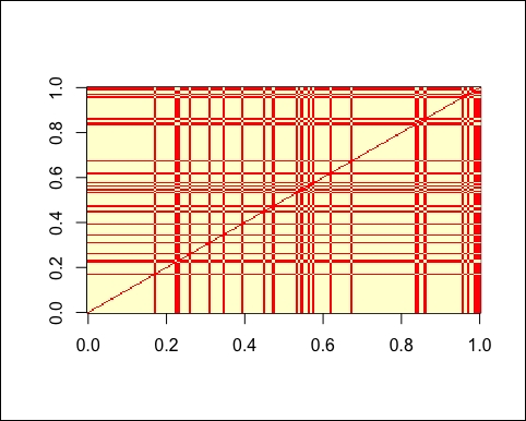
The matrix contains only 0s and 1s, and it's based on two categories, so there are clear patterns. In addition, we can notice that the matrix is symmetric.

We need to combine the two tables, and we can do it with a weighted average. Since dist_category takes account of two categories of items only, it's better not to give it too much relevance. For instance, we can set its weight to 25 percent:

weight_category <- 0.25
dist_tot <- dist_category * weight_category + dist_ratings * (1 - weight_category)

Let's take a look at the dist_tot matrix using image:

image(dist_tot)

The following image is the output of the preceding code:

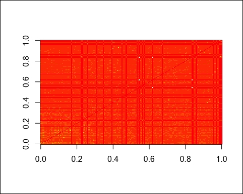
We can see some white dots representing items that are very similar. In addition, we can still see the patterns of dist_category in the background.

Now, we can include the new matrix within recc_model. For this purpose, it's sufficient to convert dist_tot into dgCMatrix and insert it in recc_model:

recc_model@model$sim <- as(dist_tot, "dgCMatrix")
recc_model@model$sim <- as(dist_tot, "dgCMatrix")

As shown in Chapter 3, Recommender Systems, we can recommend items using predict():

n_recommended <- 10
recc_predicted <- predict(object = recc_model, newdata = recc_data_test, n = n_recommended)

The itemLabels slot of recc_predicted contains the item names, that is, their code:

head(recc_predicted@itemLabels)

1038, 1026, 1034, 1008, 1056 and 1032

In order to display the item description, we can use table_items. All we need to do is make sure that the items are ordered in the same way as itemLabels. For this purpose, we will prepare a data frame containing the item information. We will also make sure that it's sorted in the same way as the item labels using the following steps:

Let's take a look at table_labels:

head(table_labels)

As expected, the table contains the description of the items. Now, we are able to extract the recommendations. For instance, we can do it for the first user:

recc_user_1 <- recc_predicted@items[[1]]
items_user_1 <- descriptions[recc_user_1]
head(items_user_1)

Windows family of OSs, Support Desktop, Knowledge Base, Microsoft.com Search, Products, and Windows 95.

Now, we can define a table with the recommendations to all users. Each column corresponds to a user and each row to a recommended item. Having set n_recommended to 10, the table should have 10 rows. For this purpose, we can use sapply() For each element of recc_predicted@items, we identify the related item descriptions.

However, the number of recommended items per user is a number between 1 and 10, which is not the same for each user. In order to define a structured table with 10 rows, we need the same number of elements for each user. For this reason, we will replace the missing recommendations with empty strings. We can obtain it by replicating the empty string with rep():

recc_matrix <- sapply(recc_predicted@items, function(x){
  recommended <- descriptions[x]
  c(recommended, rep("", n_recommended - length(recommended)))
})
dim(recc_matrix)
## _10_ and _191_

Let's take a look at the recommendations for the first three users:

head(recc_matrix[, 1:3])

We can notice that some items have been recommended to the three of them: Products and Support Desktop. Therefore, we suspect that some items are much more likely to be recommended.

Just like we did in Chapter 3, Recommender Systems, we can explore the output. For each item, we can count how many times it has been recommended:

table_recomm_per_item <- table(recc_matrix)
recomm_per_item <- as(table_recomm_per_item, "numeric")

In order to visualize the result, we bin_recomm_per_item using cut():

bin_recomm_per_item <- cut(recomm_per_item,breaks = c(0, 10, 20, 100,max(recomm_per_item)))

Using qplot, we can visualize the recomm_per_item distribution:

qplot(bin_recomm_per_item) + ggtitle("Recommendations per item")

The following image displays the recommendations per item:

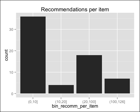
Most of the items have been recommended 10 times or fewer, and a few of them have more than 100 recommendations. The distribution has a long tail.

We can also identify the most popular items by sorting recomm_per_item:

recomm_per_item_sorted <- sort(table_recomm_per_item,decreasing = TRUE) recomm_per_item_top <- head(recomm_per_item_sorted, n = 4)
table_top <- data.frame(
  name = names(recomm_per_item_top), n_recomm = recomm_per_item_top)
table_top

In this section, we built and explored a hybrid recommender model. The next step is to evaluate it and optimize its parameters.