
For our purposes, we will define simple filters as consisting of a single filter placed on an element or attribute for the purpose of reducing the visual complexity of a network graph. The filter could be used to limit or highlight nodes, edges, partitions, or clusters in an effort to better understand and view structures within the larger network. To that end, we will devote this section to illustrate multiple examples for using simple filters to produce meaningful results that can be easily understood by the end users.
Even the so-called simple filters can help us uncover many intricacies in a network graph, particularly in cases where the network is too large to be easily deciphered by the naked eye. The following pages of examples are intended to walk you through the filtering process and provide an idea for what's possible even if you venture no further. Once again, we'll be using the primary school network to illustrate the power of simple filtering. This network can be found and downloaded from http://www.sociopatterns.org/datasets/primary-school-cumulative-networks/.
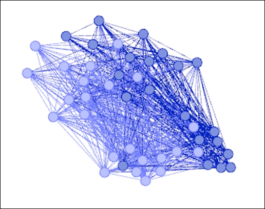
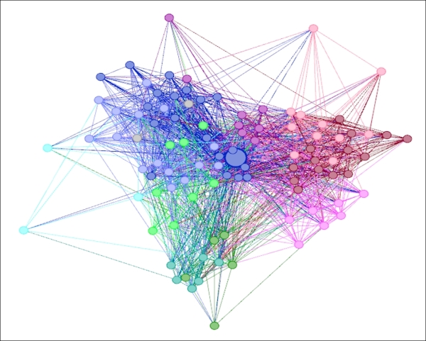
Let's start by looking at the entire network, colored by classnames:
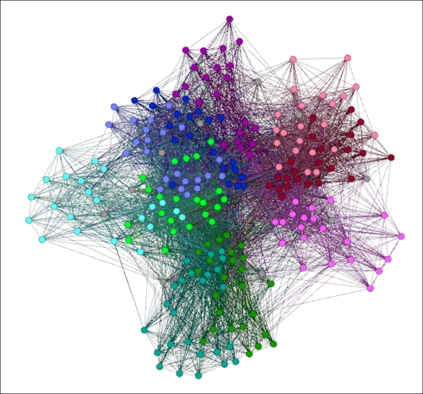
Entire primary school network
Even though this is not a large network, being composed of just 236 nodes, it still presents a visual challenge, in part due to the high degree of connectedness within the graph. We could simply choose not to show the edges, but we would then lose much of what makes the network unique. So our goal in the next few sections is to illustrate the value of filtering, not just for visual clarity, but also because we might well wind up seeing unanticipated patterns.
We'll employ a host of filters to begin navigating the graph, starting with setting the gender attribute to female, by following these simple steps:
Your query settings should look like this:
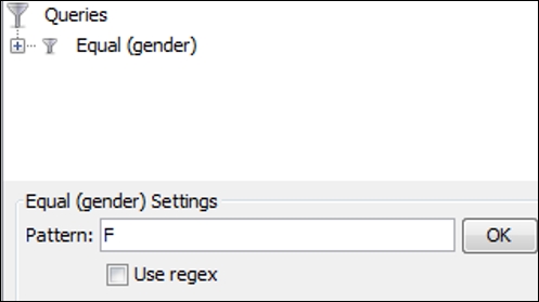
Filtering on gender using the Queries window
Here's our result after applying the filter:
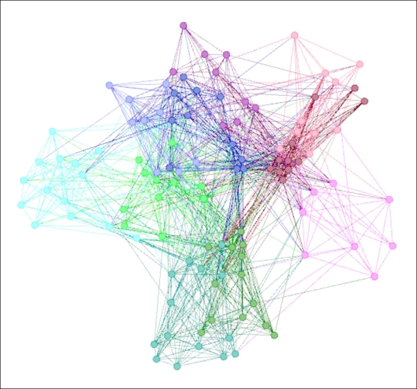
Primary school network filtered on female gender
While we haven't discovered anything too significant yet, the network has been thinned a bit which makes it somewhat easier to interpret. There are a couple of spots in the graph with very high density that might be worth investigating, but there is more we can do to query this network.
Let's remove the current filter (right-click on the filter and select Remove) and replace it with an instance where we become more selective with the data. Follow these steps to replicate the process:
- Navigate to the Filters | Attributes | Equal filter and select the
classnameattribute. - Drag the
classnameattribute to the Queries space in the lower half of the Filters tab. - Set the value to
3Band run the Select and Filter options using the available buttons.
Here's our result:
Filtering on classname equals 3B
Now, we have something we can really focus on, as we have completely removed all the remaining classnames from the display. Notice the high degree of connectedness within this group, as well as the single node at the bottom-left, positioned some distance from the other classmates. This might provide a clue that this individual is more likely to be adjacent to some other classes, or perhaps acts as a bridge between classes.
Let's move on to another example using the same approach with a single difference. Certain Gephi filters enable the use of the Regular Expressions (Regex) function, which permits wildcards as part of the filter criteria. You probably already noticed this in the prior examples, and now we will take advantage of its capabilities. If you wish to learn more about using regex, visit http://www.regular-expressions.info/.
The only change we need to make is to replace the 3B value with 3 (3 followed by a period (.) symbol), followed by checking the Use regex checkbox. Now our filter will seek any instance where the classname starts with 3, which should return both 3A and 3B (think of this as similar to a LIKE statement in a database query). This will enable us to view the entire third grade to understand how much interaction occurs both within and across the two classes. Here's our graph:
Filter with classname equal to 3. using regex
Let's switch from the Equal filter to the Inter Edges option, which will give us the opportunity to examine how nodes in one class link to those in another. To do this, we're going to remove the existing filter, and then apply the new one using the following steps:
- Navigate to the Filters | Attributes | Inter Edges filter and select the
classnameattribute. - Drag the
classnameattribute to the Queries space in the lower half of the Filters tab. - Set the values to
1Band2Bby clicking on their respective boxes and then run the Select and Filter options.
This will give us a look at the level of interaction between classrooms 1B and 2B—a single grade apart but presumably located in close proximity to one another:
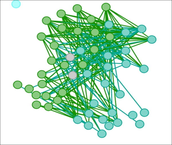
Inter Edges filter on classnames 1B and 2B
It is quite easy to see that a considerable degree of interactivity occurs across these two classrooms. Notice also that this image is merely a subset of the entire graph, and the only portion with edges on display. There are some approaches that will also remove the remaining nodes from view, which will be covered in the next section on complex filters. For now, we can zoom in for better focus on our selected classes.
We have just seen the level of connectedness across these two classes, but what about within each class? To answer this question, we will simply replace the Inter Edges filter condition with Intra Edges, using the following steps (remember to remove the existing filter first):
- Navigate to the Filters | Attributes | Intra Edges filter and select the
classnameattribute. - Drag the
classnameattribute to the Queries space in the lower half of the Filters tab. - Set the values to
1Band2Bby clicking on their respective boxes and then run the Select and Filter options.
Let's see what happens when this filter is applied:
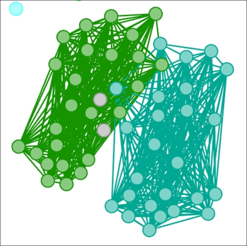
Intra Edges filter on classnames 1B and 2B
Now we get an idea for how dense each class is—at first glance, it appears that connections within each class are much stronger than those across the classes. This can be verified using various graph statistics, which we'll introduce in Chapter 6, Graph Statistics.
The Partition filter is another valuable tool that makes it very easy to select multiple values within an attribute. We'll demonstrate this in the following example. We'll begin by removing the existing filter, and then follow these steps to apply the partition conditions:
- Navigate to the Filters | Attributes | Partition filter and select the
classnameattribute. - Drag the
classnameattribute to the Queries space in the lower half of the Filters tab. - Set the values to
4A,4B,5A, and5Bby clicking on their respective boxes and then run the Select and Filter options.
This will offer a view of the higher grade levels in the school and provide a first look at their patterns with respect to one another. Let's have a look at the resultant graph:
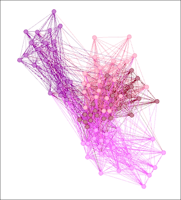
Partition filter on classnames 4A, 4B, 5A, and 5B
Here we get more interesting results, where there is some obvious overlap in the center of the graph composed of multiple classname members. Also of interest are the members at the lower-right and upper-left of the network, who appear to be less likely to interact with students from classes beyond their own.
To this point, our focus has been driven primarily by class levels. Now it's time to shift our focus to individual student behavior free from the somewhat artificial constraints of grade and class structures. This might also be a better way to understand critical behaviors within the network that are potentially being masked by group affiliations.
With that in mind, let's set our next filter using the following steps:
- Navigate to the Filters | Topology | Degree Range filter.
- Drag the filter to the Queries space in the lower half of the Filters tab.
- Use the slider control to adjust the filter, moving the left slider to a value of
80(or alternatively, type the value manually). Then run the Select and Filter options.
Our goal here is to reduce the viewable network to the most highly connected nodes so that we can observe who is most influential without having to cut through the visual clutter of seeing every member of the network. This will dramatically reduce the scope of the graph—your results should look like this:
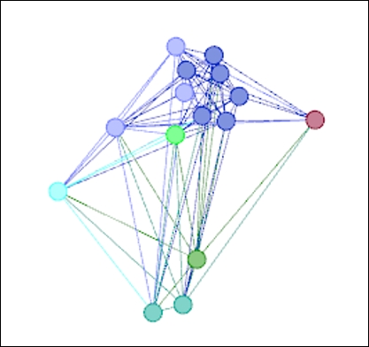
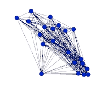
Filter on degree range from 80 to 98
This simple filter reduced our graph from 236 to just 15 nodes. There are two immediate benefits to this approach. First, we can now easily identify the most highly-connected members of the network and simultaneously identify which classname they belong to, assuming that we have elected to partition the graph based on classname (you can read more on partitioning in Chapter 7, Segmenting and Partitioning a Graph).
Secondly, we can also detect connections between these influential members, which will shed a little insight into clustering patterns in the network. It does in fact appear that a majority of these nodes are connected with one another, which some of our statistical tests in Chapter 6, Graph Statistics, should pick up. In addition, we will learn how statistics can be recalculated after filters have been applied.
Let's go through two more quick examples before we move on to more complex filters. Our first example simply adjusts the filter settings from the previous example, as we seek to learn more about the least connected members of the graph. Use the slider to adjust the filter to return nodes with degree ranges between 18 and 30, and view the results:
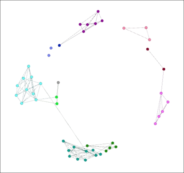
Filter on degree ranges between 18 and 30
As you might anticipate, the nodes with the lowest levels of interaction with the network are positioned around the perimeter of the graph. There are a couple of interesting patterns worth investigating from these results, with three of the classes having clusters that appear to be highly connected within the group, but are likely to have few external connections. While these don't appear to be perfect cliques where every node is interconnected, the patterns are still intriguing and can lead us to some interesting conclusions.
Our final example focuses on a single member of the network and his connections to others. Using the data laboratory, we have identified Node 1551 as the most highly connected member of the network, with a degree range equal to 98. This makes him a worthy candidate for further exploration as we attempt to understand his entire neighbor network and where they reside.
We're now going to explore the ego network for Node 1551. An ego network is simply the network of nodes that are connected to a single selected node. At a depth of one, we will see only the direct connections of the selected node, while a depth of two will show us all the second-level connections (the so-called friends of friends' network). To achieve this, we can employ the Ego Network filter, which can be applied using the following steps:
- Navigate to the Filters | Topology | Ego Network filter.
- Drag the filter to the Queries space in the lower half of the Filters tab.
- Type the value
1551in the Node ID box and leave the Depth setting equal to1. Then run the Select and Filter options to see the first degree ego network for this node.
Here are the results, with Node 1551 manually resized for easier interpretation (you could also manually recolor for a similar effect):
Ego Network for Node 1551
Now we have an instructive view into the extent of Node 1551's influence across the network. While a majority of the connections are relatively close by, there are also some outliers at the perimeter of the graph, an indication that this particular student has interacted with a wide range of other students across multiple grades and classes. This might lead us to further investigate the reasons, if any, for this pattern. A similar analysis can be performed for any other node by entering the node ID in the filter.
By now, you should have a firm grasp of what can be done using simple filters. The benefits of filtering can be enormous, especially when we are encountered with dense networks that are difficult to decipher to the networks that are easily deciphered. Now the time has come to step up to complex filters where multiple conditions are combined in a single query.