
This chapter shows how to build and train basic neural networks in R through hands-on examples that also emphasize the importance of evaluating different tuning parameters for models to find the best set. Although evaluating a variety of tuning parameters can help increase the performance of a model, it can also lead to overfitting, the next topic covered in the chapter. The chapter closes with an example use case classifying activity data from a smartphone as walking, going up or down stairs, sitting, standing, or lying down.
This chapter covers the following topics:
- Neural networks in R
- The problem of overfitting data – the consequences explained
- Use case – build and apply a neural network
To train basic (that is, "shallow" with a single hidden layer) neural networks in R, we will use the nnet and the RSNNS (Bergmeir, C., and Benítez, J. M. (2012)) packages. From the previous chapter, these should already be installed and based on a 20th February 2016 checkpoint so our results are fully reproducible. Although it is possible to interface with the nnet package directly, we are going to use it through the caret package, which is short for Classification and Regression Training. The caret package provides a standardized interface to work with many machine learning models in R (Kuhn, 2008; Kuhn and Johnson, 2013), and also has some useful features for validation and performance assessment that we will use in this chapter and the next.
For our first examples of building neural networks, we will use a classic classification problem—recognizing handwritten digits based on pictures. The data can be downloaded from https://www.kaggle.com/c/digit-recognizer and comes in an easy-to-use CSV format, where each column of the dataset, or feature, represents a pixel from the image. Each image has been normalized to a fixed size so every image has the same number of pixels. The first column contains the actual digit label, and the remaining are pixel darkness values, to be used for classification. The downloaded files, called train.csv and test.csv, were placed in the same folder as the R scripts, so they can easily be read in. If you put them in different folders, just change the paths accordingly.
To get started, we will first load our packages, by calling source() on the script where we loaded them, and set the checkpoint for the versions to use. Then we can read in the training data downloaded from
Kaggle, and take a quick look at what it is like:
source("checkpoint.R")
## output omitted
digits.train <- read.csv("train.csv")

dim(digits.train)

[1] 42000   785

head(colnames(digits.train), 4)

[1] "label"  "pixel0" "pixel1" "pixel2"

tail(colnames(digits.train), 4)

[1] "pixel780" "pixel781" "pixel782" "pixel783"

head(digits.train[, 1:4])

  label pixel0 pixel1 pixel2
1     1      0      0      0
2     0      0      0      0
3     1      0      0      0
4     4      0      0      0
5     0      0      0      0
6     0      0      0      0
We will convert the labels (the digits 0 to 9) to a factor so R knows that this is a classification not a regression problem. If this were a real-world problem, we would want to use all 42,000 observations but, for the sake of reducing how long it takes to run, we will select just the first 5,000 for these first examples of building and training a neural network. We also separate the data into the features or predictors (digits.X) and the outcome (digits.Y). We are using all the columns except the labels as the predictors here:
## convert to factor
digits.train$label <- factor(digits.train$label, levels = 0:9)
i <- 1:5000
digits.X <- digits.train[i, -1]
digits.y <- digits.train[i, 1]
Finally, before we get started building our neural network, let's quickly check the distribution of the digits. This can be important as, for example, if one digit occurs very rarely, we may need to adjust our modeling approach to ensure that, even though it is rare, it is given enough weight in performance evaluation if we care about accurately predicting that digit as well. The following code snippet creates a bar plot showing the frequency of each digit label (Figure 2.1). They are fairly evenly distributed so there is no real need to increase the weight or importance given to any particular one:
barplot(table(digits.y))

Figure 2.1
Now let's build and train our first neural network using the nnet package through the caret package wrapper. First, we use the set.seed() function and specify a specific seed so that the results are reproducible. The exact seed is not important. This same approach is also used in later examples repeating the same seed, because what matters is that the same seed is used for the same model, not whether different models have different or similar seeds. The train() function first takes the feature or predictor data, the x argument, and then the outcome variable, the y argument. The train() function can work with a variety of models, determined via the method argument. Although many aspects of machine learning models are learned automatically, some parameters have to be set. These vary by the method used; for example, in neural networks one parameter is the number of hidden units. The train() function provides an easy way to try a variety of these tuning parameters as a named data frame to the tuneGrid argument. It returns the performance measures for each set of tuning parameters and returns the best trained model. We will start with just five hidden neurons in our model, and a modest decay rate, sometimes also called the
learning rate. The learning rate controls how much each iteration or step can influence the current weights. Another argument, trControl, controls additional aspects of train(), and is used, when a variety of tuning parameters are being evaluated, to tell the caret package how to validate and pick the best tuning parameter.
For this example, we will set the method for training control to "none" as we only have one set of tuning parameters being used here. Finally, at the end we can specify additional, named arguments that are passed on to the actual nnet() function (or whatever algorithm is specified). Because of the number of predictors (784), we increase the maximum number of weights to 10,000 and specify a maximum of 100 iterations. Due to the relatively small amount of data, and the paucity of hidden neurons, this first model does not take too long to run:
set.seed(1234)
digits.m1 <- train(x = digits.X, y = digits.y,
           method = "nnet",
           tuneGrid = expand.grid(
             .size = c(5),
             .decay = 0.1),
           trControl = trainControl(method = "none"),
           MaxNWts = 10000,
           maxit = 100)
The predict() function generates a set of predictions for data. When called on the results of a model without specifying any new data, it just generates predictions on the same data used for training. After calculating and storing the predicted digits, we can examine their distribution, shown in Figure 2.2. Even before looking at the performance measures for this first model, given the actual distribution (Figure 2.1) it is clear this model is not optimal:
digits.yhat1 <- predict(digits.m1)
barplot(table(digits.yhat1))

Figure 2.2
Graphically examining the distribution is just a simple check of the predictions. A more formal evaluation of model performance is possible using the confusionMatrix() function in the caret package. Because there is a function by the same name in the RSNNS package, they are masked so we use the special caret:: code to tell R which version of the function to use. The input is simply a frequency cross tab between the actual digits and the predicted digits. The remaining performance metrics are calculated from these.
Because we had multiple digits, there are three main sections to the performance output. First, the actual frequency cross tab is shown. Correct predictions are on the diagonal, with various frequencies of misclassification on the off diagonals. Next are the overall statistics, which refer to the model performance across all classes. Accuracy is simply the proportion of cases correctly classified, along with a 95% confidence interval, which can be useful especially for smaller datasets where there may be considerable uncertainty in the estimate. The No Information Rate refers to what accuracy could be expected without any information by merely guessing the most frequent class, in this case, 1, which occurred 11.16% of the time. The p-value tests whether the observed accuracy (44.3%) is significantly different than the No Information Rate (11.2%). Although statistically significant, this is not very meaningful for digit classification where we would expect to do far better than simply guessing the most frequent digit! Finally, individual performance metrics for each digit are shown. These are based on calculating that digit versus every other digit, so that each is a binary comparison. The following 2 x 2 table contains all the information needed to calculate the various measures, and the formulae for all the measures are shown here:
|
Positive |
Negative | |
|---|---|---|
|
Predicted positive |
True positive (TP) |
False positive (FP) |
|
Predicted negative |
False negative (FN) |
True negative (TN) |


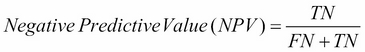


For example, the sensitivity for digit 0 can be interpreted as meaning that 78.5% of zero digits were captured or correctly predicted to be zeroes. The specificity for digit 0 can be interpreted as meaning that 95.2% of cases that were predicted to be a digit other than zero were not zero. The detection rate is just the percentage of true positives, and finally the detection prevalence is the proportion of cases predicted to be positive, regardless of whether they actually are or not. The balanced accuracy is the mean of the sensitivity and specificity. The remaining columns present the same information for each of the remaining digits:
caret::confusionMatrix(xtabs(~digits.yhat1 + digits.y))

Confusion Matrix and Statistics

            digits.y
digits.yhat1   0   1   2   3   4   5   6   7   8   9
           0 388   2  40  41   7  75  23   4  23   2
           1   0 495   3   0   0   3   0   4   3   4
           2   0   0   0   0   0   0   0   0   0   0
           3  51  30  36 379   6 329   3  18 290  38
           4   0   0   0   0   0   0   0   0   0   0
           5   0   0   0   0   0   0   0   0   0   0
           6  44   5 304   9 131  29 484   9  16  19
           7  11  26 162  51 333  33   6 470 145 415
           8   0   0   0   0   0   0   0   0   0   0
           9   0   0   0   0   0   0   0   1   0   0

Overall Statistics

               Accuracy : 0.4432
                 95% CI : (0.4294, 0.4571)
    No Information Rate : 0.1116
    P-Value [Acc > NIR] : < 2.2e-16

                  Kappa : 0.3805
 Mcnemar's Test P-Value : NA

Statistics by Class:

                     Class: 0 Class: 1 Class: 2 Class: 3 Class: 4
Sensitivity            0.7854   0.8871    0.000   0.7896   0.0000
Specificity            0.9518   0.9962    1.000   0.8228   1.0000
Pos Pred Value         0.6413   0.9668      NaN   0.3212      NaN
Neg Pred Value         0.9759   0.9860    0.891   0.9736   0.9046
Prevalence             0.0988   0.1116    0.109   0.0960   0.0954
Detection Rate         0.0776   0.0990    0.000   0.0758   0.0000
Detection Prevalence   0.1210   0.1024    0.000   0.2360   0.0000
Balanced Accuracy      0.8686   0.9416    0.500   0.8062   0.5000
                     Class: 5 Class: 6 Class: 7 Class: 8 Class: 9
Sensitivity            0.0000   0.9380   0.9289   0.0000   0.0000
Specificity            1.0000   0.8738   0.7370   1.0000   0.9998
Pos Pred Value            NaN   0.4610   0.2845      NaN   0.0000
Neg Pred Value         0.9062   0.9919   0.9892   0.9046   0.9044
Prevalence             0.0938   0.1032   0.1012   0.0954   0.0956
Detection Rate         0.0000   0.0968   0.0940   0.0000   0.0000
Detection Prevalence   0.0000   0.2100   0.3304   0.0000   0.0002
Balanced Accuracy      0.5000   0.9059   0.8329   0.5000   0.4999
Now that we have some basic understanding of how to set up, train, and evaluate model performance, we will try a few different models, increasing the number of hidden neurons, which is one key way to improve model performance, at the cost of greatly increasing the model complexity. Recall from Chapter 1, Getting Started with Deep Learning, that every predictor or feature connects to each hidden neuron, and each hidden neuron connects to each outcome or output. With 784 features, each additional hidden neuron adds a substantial number of parameters, which also results in longer run times. Depending on your computer, be prepared to wait a number of minutes for these next models to finish:
set.seed(1234)
digits.m2 <- train(digits.X, digits.y,
           method = "nnet",
           tuneGrid = expand.grid(
             .size = c(10),
             .decay = 0.1),
           trControl = trainControl(method = "none"),
            MaxNWts = 50000,
            maxit = 100)

digits.yhat2 <- predict(digits.m2)
barplot(table(digits.yhat2))
Figure 2.3
caret::confusionMatrix(xtabs(~digits.yhat2 + digits.y))

Confusion Matrix and Statistics

            digits.y
digits.yhat2   0   1   2   3   4   5   6   7   8   9
           0 395   0  14  23   0 120   6  12  15   5
           1   2 518  35  10   0   7   0  10   8   4
           2  23  23 323  15   8  37  30   1  15   2
           3   0   4  24 337   0  49   0  12  37   5
           4   3   0   0   0  10  14   2   0   0   0
           5  44   0  20  60   0 146  10   1 235   9
           6   1   1  25   2   0   3 327   0   3   0
           7   3   1   7   3   3  11   7 392   3  19
           8   0   0   0   0   0   0   1   0   0   0
           9  23  11  97  30 456  82 133  78 161 434

Overall Statistics

               Accuracy : 0.5764
                 95% CI : (0.5626, 0.5901)
    No Information Rate : 0.1116
    P-Value [Acc > NIR] : < 2.2e-16

                  Kappa : 0.5293
 Mcnemar's Test P-Value : NA

Statistics by Class:

                     Class: 0 Class: 1 Class: 2 Class: 3 Class: 4
Sensitivity            0.7996   0.9283   0.5927   0.7021  0.02096
Specificity            0.9567   0.9829   0.9654   0.9710  0.99580
Pos Pred Value         0.6695   0.8721   0.6771   0.7201  0.34483
Neg Pred Value         0.9776   0.9909   0.9509   0.9684  0.90606
Prevalence             0.0988   0.1116   0.1090   0.0960  0.09540
Detection Rate         0.0790   0.1036   0.0646   0.0674  0.00200
Detection Prevalence   0.1180   0.1188   0.0954   0.0936  0.00580
Balanced Accuracy      0.8782   0.9556   0.7790   0.8366  0.50838
                     Class: 5 Class: 6 Class: 7 Class: 8 Class: 9
Sensitivity            0.3113   0.6337   0.7747   0.0000   0.9079
Specificity            0.9164   0.9922   0.9873   0.9998   0.7632
Pos Pred Value         0.2781   0.9033   0.8731   0.0000   0.2884
Neg Pred Value         0.9278   0.9592   0.9750   0.9046   0.9874
Prevalence             0.0938   0.1032   0.1012   0.0954   0.0956
Detection Rate         0.0292   0.0654   0.0784   0.0000   0.0868
Detection Prevalence   0.1050   0.0724   0.0898   0.0002   0.3010
Balanced Accuracy      0.6138   0.8130   0.8810   0.4999   0.8356
Increasing from 5 to 10 hidden neurons improved our in-sample performance from an overall accuracy of 44.3% to 57.6%, but this is still quite some way from ideal (imagine character recognition software that mixed up 42.4% of all the characters!). We increase again, this time to 40 hidden neurons, and wait even longer for the model to finish training:
set.seed(1234)
digits.m3 <- train(digits.X, digits.y,
           method = "nnet",
           tuneGrid = expand.grid(
             .size = c(40),
             .decay = 0.1),
           trControl = trainControl(method = "none"),
           MaxNWts = 50000,
           maxit = 100)

digits.yhat3 <- predict(digits.m3)
barplot(table(digits.yhat3))
Figure 2.4
caret::confusionMatrix(xtabs(~digits.yhat3 + digits.y))

Confusion Matrix and Statistics

            digits.y
digits.yhat3   0   1   2   3   4   5   6   7   8   9
           0 461   0   7   3   0  20  16   2   3   7
           1   0 521   3   4   0   2   2   6  10   2
           2  17   3 469  30   2  13  16  10  39   2
           3   1   5  11 352   2  43   2   9  48   5
           4   1   0   6   1 394   7   0   4   3  36
           5   3   4   2  23   1 334  12   1  51   6
           6   6   1  19   3  15  10 455   1   3   1
           7   0   2   8   7   5   5   2 411   6  35
           8   2  20  10  46   4  28   9  10 297  23
           9   3   2  10  11  54   7   2  52  17 361

Overall Statistics

               Accuracy : 0.811
                 95% CI : (0.7999, 0.8218)
    No Information Rate : 0.1116
    P-Value [Acc > NIR] : < 2.2e-16

                  Kappa : 0.7899
 Mcnemar's Test P-Value : NA

Statistics by Class:

                     Class: 0 Class: 1 Class: 2 Class: 3 Class: 4
Sensitivity            0.9332   0.9337   0.8606   0.7333   0.8260
Specificity            0.9871   0.9935   0.9704   0.9721   0.9872
Pos Pred Value         0.8882   0.9473   0.7804   0.7364   0.8717
Neg Pred Value         0.9926   0.9917   0.9827   0.9717   0.9818
Prevalence             0.0988   0.1116   0.1090   0.0960   0.0954
Detection Rate         0.0922   0.1042   0.0938   0.0704   0.0788
Detection Prevalence   0.1038   0.1100   0.1202   0.0956   0.0904
Balanced Accuracy      0.9602   0.9636   0.9155   0.8527   0.9066
                     Class: 5 Class: 6 Class: 7 Class: 8 Class: 9
Sensitivity            0.7122   0.8818   0.8123   0.6226   0.7552
Specificity            0.9773   0.9868   0.9844   0.9664   0.9651
Pos Pred Value         0.7643   0.8852   0.8545   0.6615   0.6956
Neg Pred Value         0.9704   0.9864   0.9790   0.9604   0.9739
Prevalence             0.0938   0.1032   0.1012   0.0954   0.0956
Detection Rate         0.0668   0.0910   0.0822   0.0594   0.0722
Detection Prevalence   0.0874   0.1028   0.0962   0.0898   0.1038
Balanced Accuracy      0.8447   0.9343   0.8983   0.7945   0.8601
Using 40 hidden neurons has improved performance dramatically again, up to 81.1% overall. Model performance for 3s, 5s, 8s, and 9s is still not great, but the remaining digits are quite good. If this were a real research or business problem, we might continue trying additional neurons, tuning the decay rate, or modifying features in order to try to boost model performance further, but for now we will move on.
Next, we will take a look at how to train neural networks using the RSNNS package. This package provides an interface to quite a variety of possible models using the Stuttgart Neural Network Simulator (SNNS) code; however, for a basic, single-hidden-layer, feed-forward neural network, we can use the mlp() convenience wrapper function, which stands for multi-layer perceptron. The RSNNS package is a bit more finicky to use than the convenience of nnet via the caret package, but one benefit is that it can be far more flexible and allows for many other types of neural network architectures to be trained, including recurrent neural networks, and also has a greater variety of learning functions.
One difference between the nnet and RSNNS package is that for multi-class outcomes (such as digits), RSNNS requires a dummy coded matrix, so each possible class is represented as a column coded as 0/1. This is facilitated using the decodeClassLabels() function, and a bit of the output is shown next:
head(decodeClassLabels(digits.y))

     0 1 2 3 4 5 6 7 8 9
[1,] 0 1 0 0 0 0 0 0 0 0
[2,] 1 0 0 0 0 0 0 0 0 0
[3,] 0 1 0 0 0 0 0 0 0 0
[4,] 0 0 0 0 1 0 0 0 0 0
[5,] 1 0 0 0 0 0 0 0 0 0
[6,] 1 0 0 0 0 0 0 0 0 0
Since we had reasonably good success with 40 hidden neurons, we will use the same size here. Rather than standard propagation as the learning function, we will use resilient propagation, based on the classic work of Riedmiller, M., and Braun, H. (1993). Note also that, because a matrix of outcomes is passed, although the predicted probability will not exceed 1 for any single digit, the sum of predicted probabilities across all digits may exceed 1 and also may be less than 1 (that is, for some cases, the model may not predict they are very likely to represent any of the digits). As before, we can get in-sample predictions, but here we have to use another function, fitted.values(). Because this again returns a matrix where each column represents a single digit, we use the encodeClassLabels() function to convert back into a single vector of digit labels to plot (Figure 2.5) and evaluate model performance:
set.seed(1234)
digits.m4 <- mlp(as.matrix(digits.X),
             decodeClassLabels(digits.y),
             size = 40,
             learnFunc = "Rprop",
             shufflePatterns = FALSE,
             maxit = 60)
digits.yhat4 <- fitted.values(digits.m4)
digits.yhat4 <- encodeClassLabels(digits.yhat4)
barplot(table(digits.yhat4))
Figure 2.5
Once we have the predicted probabilities, evaluating model performance is virtually the same as when using the nnet and caret packages. The only catch is that, when the output is encoded back into a single vector, by default the digits are labeled 1 to k, where k is the number of classes. Because the digits are 0 to 9, to make them match the original digit vector, we subtract 1. Next we can see that, using the learning algorithms from the RSNNS package, we obtained a somewhat higher performance with the same number of hidden neurons. Next we turn to generating predictions for out-of-sample data:
caret::confusionMatrix(xtabs(~ I(digits.yhat4 - 1) + digits.y))

Confusion Matrix and Statistics

                   digits.y
I(digits.yhat4 - 1)   0   1   2   3   4   5   6   7   8   9
                  0 451   0   0   1   0   2   3   2   1   1
                  1   0 534   4   2   3   1   0   7  11   2
                  2   6   3 496  17   3   4   2   4  20   1
                  3   9   5  11 406   3  21   0   2  13  10
                  4   2   1   6   0 415   7   4   4   9  24
                  5  12   2   0  14   3 376   8   4  23  13
                  6   4   4   2   2   3  12 493   2   9   1
                  7   3   0  10   7   4   1   1 460   1  37
                  8   5   9  14  28  12  31   5   8 375  13
                  9   2   0   2   3  31  14   0  13  15 376

Overall Statistics

               Accuracy : 0.8764
                 95% CI : (0.867, 0.8854)
    No Information Rate : 0.1116
    P-Value [Acc > NIR] : < 2.2e-16

                  Kappa : 0.8626
 Mcnemar's Test P-Value : NA

Statistics by Class:

                     Class: 0 Class: 1 Class: 2 Class: 3 Class: 4
Sensitivity            0.9130   0.9570   0.9101   0.8458   0.8700
Specificity            0.9978   0.9932   0.9865   0.9836   0.9874
Pos Pred Value         0.9783   0.9468   0.8921   0.8458   0.8792
Neg Pred Value         0.9905   0.9946   0.9890   0.9836   0.9863
Prevalence             0.0988   0.1116   0.1090   0.0960   0.0954
Detection Rate         0.0902   0.1068   0.0992   0.0812   0.0830
Detection Prevalence   0.0922   0.1128   0.1112   0.0960   0.0944
Balanced Accuracy      0.9554   0.9751   0.9483   0.9147   0.9287
                     Class: 5 Class: 6 Class: 7 Class: 8 Class: 9
Sensitivity            0.8017   0.9554   0.9091   0.7862   0.7866
Specificity            0.9826   0.9913   0.9858   0.9724   0.9823
Pos Pred Value         0.8264   0.9267   0.8779   0.7500   0.8246
Neg Pred Value         0.9795   0.9949   0.9897   0.9773   0.9776
Prevalence             0.0938   0.1032   0.1012   0.0954   0.0956
Detection Rate         0.0752   0.0986   0.0920   0.0750   0.0752
Detection Prevalence   0.0910   0.1064   0.1048   0.1000   0.0912
Balanced Accuracy 0.8921 0.9734 0.9474 0.8793 0.8845Up until now, we have only generated in-sample predictions on the same data used to train the neural network, and we have accepted all the defaults for obtaining the classifications. However, there are actually several options, even once the model is trained. For any given observation, there can be a probability of membership in any of a number of classes (for example, an observation may have a 40% chance of being a "5", a 20% chance of being a "6", and so on). For evaluating the performance of the model, some choices have to be made about how to go from the probability of class membership to a discrete classification. In this section, we will explore a few of these options in more detail, and also take a look at generating predictions on data not used for training.
So long as there are no perfect ties, the simplest method may be to classify observations based on the high predicted probability. Another approach, which the RSNNS package calls the winner takes all (WTA) method, is to choose the class with the highest probability so long as there are no ties, the highest probability is above a user-defined threshold (the threshold could be zero), and the remaining classes all have a predicted probability under the maximum minus another user-defined threshold. Otherwise, observations are classified as unknown. If both thresholds are zero (the default), this equates to saying that there must be one unique maximum. The advantage of such an approach is that it provides some quality control. In the digit classification example we have been exploring, there are 10 possible classes. Suppose nine of the digits had a predicted probability of 0.099, and the remaining class had a predicted probability of 0.109. Although one class is technically more likely than the others, the difference is fairly trivial and we may conclude that the model cannot with any certainty classify that observation. A final method, called 402040, classifies if only one value is above a user-defined threshold, and all other values are below another user-defined threshold; if multiple values are above the first threshold, or any value is not below the second threshold, it treats the observation as unknown. Again, the goal here is to provide some quality control. It may seem like this is unnecessary because uncertainty in predictions should come out in the model performance. However, it can be helpful to know if your model was highly certain in its prediction and right or wrong, or uncertain and right or wrong.
Finally, in some cases not all classes are equally important. For example, in a medical context where a variety of biomarkers and genes are collected on patients and used to classify whether they are healthy or not, at risk of cancer, or at risk of heart disease, even a 40% chance of having cancer may be enough to warrant further investigation, even if they have a 60% chance of being healthy. This has to do with the performance measures we saw earlier where, beyond overall accuracy, we can assess aspects such as sensitivity, specificity, and positive and negative predictive values. There are cases where overall accuracy is less important than making sure no one is missed.
The following code shows the raw probabilities for the in-sample data, and the impact these different choices have on the predicted values:
digits.yhat4.insample <- fitted.values(digits.m4)
head(round(digits.yhat4.insample, 2))

     [,1] [,2] [,3] [,4] [,5] [,6] [,7] [,8] [,9] [,10]
[1,] 0.00 0.89 0.00 0.01 0.00 0.00 0.00 0.00 0.21     0
[2,] 0.99 0.00 0.00 0.02 0.00 0.00 0.00 0.01 0.00     0
[3,] 0.00 1.00 0.09 0.00 0.00 0.00 0.00 0.05 0.00     0
[4,] 0.00 0.00 0.00 0.00 0.22 0.00 0.02 0.05 0.00     0
[5,] 1.00 0.00 0.02 0.00 0.00 0.00 0.00 0.00 0.00     0
[6,] 0.99 0.00 0.00 0.00 0.00 0.06 0.00 0.00 0.00     0

table(encodeClassLabels(digits.yhat4.insample,
                        method = "WTA", l = 0, h = 0))

  1   2   3   4   5   6   7   8   9  10
461 564 556 480 472 455 532 524 500 456

table(encodeClassLabels(digits.yhat4.insample,
                        method = "WTA", l = 0, h = .5))

  0   1   2   3   4   5   6   7   8   9  10
569 448 544 497 400 429 366 499 463 379 406

table(encodeClassLabels(digits.yhat4.insample,
                        method = "WTA", l = .2, h = .5))

  0   1   2   3   4   5   6   7   8   9  10
658 443 542 490 393 408 358 493 460 364 391

table(encodeClassLabels(digits.yhat4.insample,
                        method = "402040", l = .4, h = .6))

  0   1   2   3   4   5   6   7   8   9  10
907 431 526 472 363 383 326 475 448 301 368
We can easily generate predicted values for new data using the predict() function. For this, we will use the next 5,000 observations. Note that even generating these predictions took a couple of minutes on a new desktop:
i2 <- 5001:10000
digits.yhat4.pred <- predict(digits.m4,
                             as.matrix(digits.train[i2, -1]))

table(encodeClassLabels(digits.yhat4.pred,
                        method = "WTA", l = 0, h = 0))

  1   2   3   4   5   6   7   8   9  10
449 570 531 518 476 442 522 533 468 491
Having generated predictions on out-of-sample data (that is, data that was not used to train the model), we can now proceed to examine problems related to overfitting the data and the impact on the evaluation of model performance.