For more information on tuning hyperparameters, see Bengio, Y. (2012), particularly Section 3, Hyper-Parameters, which discusses the selection and characteristics of various hyperparameters. Aside from manual trial and error, two other approaches to improving hyperparameters are grid searches and random searches. In a grid search, several values for hyperparameters are specified and all possible combinations are tried. This is perhaps easiest to see. In R we can use the expand.grid() function to create all possible combinations of variables:

expand.grid(
  layers = c(1, 2, 4),
  epochs = c(50, 100),
  l1 = c(.001, .01, .05))

   layers epochs    l1
1       1     50 0.001
2       2     50 0.001
3       4     50 0.001
4       1    100 0.001
5       2    100 0.001
6       4    100 0.001
7       1     50 0.010
8       2     50 0.010
9       4     50 0.010
10      1    100 0.010
11      2    100 0.010
12      4    100 0.010
13      1     50 0.050
14      2     50 0.050
15      4     50 0.050
16      1    100 0.050
17      2    100 0.050
18      4    100 0.050

Grid searching is excellent when there are only a few values for a few parameters. However, although this is a comprehensive way of assessing different parameter values, when there are many values for some or many parameters, it quickly becomes unfeasible. For example, even with only two values for each of eight parameters, there are 2⁸ = 256 combinations, which quickly becomes computationally impracticable. In addition, if there are no interactions between parameters and model performance, or at least the interactions are small relative to the main effects, then grid searches are an inefficient approach because many parameter values are repeated so that only a small set of values is sampled, even though many combinations are tried.

An alternative approach is searching through random sampling. Rather than pre-specifying all the values to try and creating all possible combinations, one can randomly sample values for the parameters, fit a model, store the results, and repeat. To get a very large sample size, this too would be computationally demanding, but does make it straightforward to specify just how many different models you are willing to run.

For random sampling, all that needs to be specified are the values to randomly sample or distributions to randomly draw from. Typically, some limits would also be set. For example, although a model could theoretically have any integer number of layers, some reasonable number (such as 1 to 10) is used rather than sampling integers from 1 to a billion.

To do random sampling, we will write a function that takes a seed and then randomly samples a number of hyperparameters, stores the sampled parameters, runs the model, and returns the results. Even though we are doing a random search to try to find better values, we are not sampling from every possible hyperparameter. Many remain fixed at values we specify or their defaults.

For some parameters, specifying how to randomly sample values can take a bit of work. For example, when using dropout for regularization, it is common to have a relatively smaller amount of dropout for the input variables (around 20% commonly) and a higher amount for hidden neurons (around 50% commonly). Choosing the right distributions can allow us to encode this prior information into our random search. The following code plots the density of two beta distributions, and the results are shown in Figure 6.2. By sampling from these distributions, we can ensure that our search, while random, focuses on small proportions of dropout for the input variables and in the 0 to 0.50 range for the hidden neurons with a tendency to over-sample from values closer to 0.50:

par(mfrow = c(2, 1))
plot(
  seq(0, .5, by = .001),
  dbeta(seq(0, .5, by = .001), 1, 12),
  type = "l", xlab = "x", ylab = "Density",
  main = "Density of a beta(1, 12)")

plot(
  seq(0, 1, by = .001)/2,
  dbeta(seq(0, 1, by = .001), 1.5, 1),
  type = "l", xlab = "x", ylab = "Density",
  main = "Density of a beta(1.5, 1) / 2")

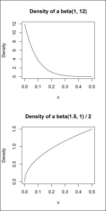
Figure 6.2

Now we can write our function, called run(). All it requires is a seed, which is used to make the parameter selection reproducible. A name can be specified, although there is a default based on the seed, and there is an optional (logical) argument, run, to control whether or not the model is run. This can be helpful if you want to check the hyperparameter values sampled.

We sample the depth or number of layers from 1 to 5 and the number of neurons in each layer from 20 to 600; by default each will have an equal probability. The runif() function samples from a uniform distribution in the specified range, and we have already seen the beta distribution, which we sample from using the rbeta() function.

Two new arguments we also randomly sample are rho and epsilon. These are used because, rather than specifying the learning rate and momentum manually, we are using (as H2O does by default) the ADADELTA algorithm (Zeiler, M. D. (2012)) to automatically tune the learning rate. ADADELTA only has two hyperparameters that need to be specified: rho and epsilon. ADADELTA works in part by examining the previous gradients but, rather than store all previous gradients, a weighted cumulative average is used. The rho parameter is used to weight the gradients prior to the current iteration and 1 – rho is used to weight the gradient at the current iteration. If rho = 1, then the current gradient is not used and it is completely based on the previous gradients. If rho = 0, the previous gradients are not used and it is completely based on the current gradient. Typically, values between .9 and .999 are used.

The epsilon parameter is a small constant that is added when taking the root mean square of previous squared gradients to improve conditioning (it is ideal to avoid this becoming actually zero) and is typically a very small number. Further details are available from the paper presenting ADADELTA (Zeiler, M. D. (2012)):

run <- function(seed, name = paste0("m_", seed), run = TRUE) {
  set.seed(seed)

  p <- list(
    Name = name,
    seed = seed,
    depth = sample(1:5, 1),
    l1 = runif(1, 0, .01),
    l2 = runif(1, 0, .01),
    input_dropout = rbeta(1, 1, 12),
    rho = runif(1, .9, .999),
    epsilon = runif(1, 1e-10, 1e-4))

  p$neurons <- sample(20:600, p$depth, TRUE)
  p$hidden_dropout <- rbeta(p$depth, 1.5, 1)/2

  if (run) {
  model <- h2o.deeplearning(
    x = colnames(use.train.x),
    y = "Outcome",
    training_frame = h2oactivity.train,
    activation = "RectifierWithDropout",
    hidden = p$neurons,
    epochs = 100,
    loss = "CrossEntropy",
    input_dropout_ratio = p$input_dropout,
    hidden_dropout_ratios = p$hidden_dropout,
    l1 = p$l1,
    l2 = p$l2,
    rho = p$rho,
    epsilon = p$epsilon,
    export_weights_and_biases = TRUE,
    model_id = p$Name
  )

  ## performance on training data
  p$MSE <- h2o.mse(model)
  p$R2 <- h2o.r2(model)
  p$Logloss <- h2o.logloss(model)
  p$CM <- h2o.confusionMatrix(model)

  ## performance on testing data
  perf <- h2o.performance(model, h2oactivity.test)
  p$T.MSE <- h2o.mse(perf)
  p$T.R2 <- h2o.r2(perf)
  p$T.Logloss <- h2o.logloss(perf)
  p$T.CM <- h2o.confusionMatrix(perf)

  } else {
    model <- NULL
  }

  return(list(
    Params = p,
    Model = model))
}

Before we can run the models, we need to load our data, which for this example is the activity data:

use.train.x <- read.table("UCI HAR Dataset/train/X_train.txt")
use.test.x <- read.table("UCI HAR Dataset/test/X_test.txt")

use.train.y <- read.table("UCI HAR Dataset/train/y_train.txt")[[1]]
use.test.y <- read.table("UCI HAR Dataset/test/y_test.txt")[[1]]

use.train <- cbind(use.train.x, Outcome = factor(use.train.y))
use.test <- cbind(use.test.x, Outcome = factor(use.test.y))

use.labels <- read.table("UCI HAR Dataset/activity_labels.txt")

h2oactivity.train <- as.h2o(
  use.train,
  destination_frame = "h2oactivitytrain")

h2oactivity.test <- as.h2o(
  use.test,
  destination_frame = "h2oactivitytest")

In order to make the parameters reproducible, we specify a list of random seeds, which we loop through to run the models:

use.seeds <- c(403L, 10L, 329737957L, -753102721L, 1148078598L, -1945176688L,
-1395587021L, -1662228527L, 367521152L, 217718878L, 1370247081L,
571790939L, -2065569174L, 1584125708L, 1987682639L, 818264581L,
1748945084L, 264331666L, 1408989837L, 2010310855L, 1080941998L,
1107560456L, -1697965045L, 1540094185L, 1807685560L, 2015326310L,
-1685044991L, 1348376467L, -1013192638L, -757809164L, 1815878135L,
-1183855123L, -91578748L, -1942404950L, -846262763L, -497569105L,
-1489909578L, 1992656608L, -778110429L, -313088703L, -758818768L,
-696909234L, 673359545L, 1084007115L, -1140731014L, -877493636L,
-1319881025L, 3030933L, -154241108L, -1831664254L)

The models can be run (although it takes some time) simply by looping through the seeds:

model.res <- lapply(use.seeds, run)

Once the models are done, we can create a dataset, and plot the mean squared error (MSE) against the different parameters, using the following code. The results are shown in Figure 6.3:

model.res.dat <- do.call(rbind, lapply(model.res, function(x) with(x$Params,
  data.frame(l1 = l1, l2 = l2,
             depth = depth, input_dropout = input_dropout,
             SumNeurons = sum(neurons),
             MeanHiddenDropout = mean(hidden_dropout),
             rho = rho, epsilon = epsilon, MSE = T.MSE))))


p.perf <- ggplot(melt(model.res.dat, id.vars = c("MSE")), aes(value, MSE)) +
  geom_point() +
  stat_smooth(color = "black") +
  facet_wrap(~ variable, scales = "free_x", ncol = 2) +
  theme_classic()
print(p.perf)

Figure 6.3

In addition to viewing the univariate relations between parameters and the model error, it can be helpful to use a multivariate model to simultaneously take different parameters into account.

To fit this (and allow some non-linearity), we use a generalized additive model, using the gam() function from the mgcv package. We specifically hypothesize an interaction between the model depth and total number of hidden neurons, which we capture by including both of those terms in a tensor expansion using the te() function, with the remaining terms given univariate smooths, using the s() function. The specifics here are not so important. The key is to somehow model the relation between the hyperparameters and model performance in order to decide what values should be chosen:

m.gam <- gam(MSE ~ s(l1, k = 4) +
              s(l2, k = 4) +
              s(input_dropout) +
              s(rho, k = 4) +
              s(epsilon, k = 4) +
              s(MeanHiddenDropout, k = 4) +
              te(depth, SumNeurons, k = 4),
            data = model.res.dat)

Now we can visualize the results. The first six univariate terms we plot on one graph, using the following code; this is shown in Figure 6.4. The constant term is not shown, so these values are not directly MSE estimates, but the key is to find the lowest point for each hyperparameter:

par(mfrow = c(3, 2))
for (i in 1:6) {
  plot(m.gam, select = i)
}

Figure 6.4

Finally, we plot the interaction term with the following code:

plot(m.gam, select = 7)

The results are shown in Figure 6.5. This is a contour plot and shows each variable in the interaction on the x and y axes. The actual MSE is not shown, but is labeled on the lines. Because of the interaction, it is possible to get the same estimated MSE using different combinations of the predictors. In general, it seems that, the more layers there are, the more neurons are required to achieve a comparable performance:

Figure 6.5

Based on these graphs, we chose hyperparameters and specify an optimized model in the following code:

model.optimized <- h2o.deeplearning(
    x = colnames(use.train.x),
    y = "Outcome",
    training_frame = h2oactivity.train,
    activation = "RectifierWithDropout",
    hidden = c(300, 300, 300),
    epochs = 100,
    loss = "CrossEntropy",
    input_dropout_ratio = .08,
    hidden_dropout_ratios = c(.50, .50, .50),
    l1 = .002,
    l2 = 0,
    rho = .95,
    epsilon = 1e-10,
    export_weights_and_biases = TRUE,
    model_id = "optimized_model"
)

After training, we can estimate the model performance in the validation data by using the h2o.performance() function and passing the optimized model and the testing data as arguments:

H2OMultinomialMetrics: deeplearning

Test Set Metrics: 
=====================

MSE: (Extract with `h2o.mse`) 0.053
R^2: (Extract with `h2o.r2`) 0.98
Logloss: (Extract with `h2o.logloss`) 0.18
Confusion Matrix: Extract with `h2o.confusionMatrix(<model>, <data>)`)
=========================================================================
        X1  X2  X3  X4  X5  X6 Error        Rate
1      491   0   5   0   0   0 0.010     5 / 496
2       12 457   1   0   1   0 0.030    14 / 471
3       32  47 341   0   0   0 0.188    79 / 420
4        0   2   0 434  55   0 0.116    57 / 491
5        0   0   0  38 494   0 0.071    38 / 532
6        0   0   0   0  15 522 0.028    15 / 537
Totals 535 506 347 472 565 522 0.071 208 / 2,947

Hit Ratio Table: Extract with `h2o.hit_ratio_table(<model>, <data>)`
=======================================================================
Top-6 Hit Ratios: 
  k hit_ratio
1 1  0.929420
2 2  0.993892
3 3  0.998643
4 4  0.999661
5 5  1.000000
6 6  1.000000

Finally, we can compare the performance of our optimized model against the single best model from the random search. Using the optimized parameters, we were able to achieve an MSE of 0.053 in the testing data, a reduction of approximately 21% from the single best model found during the random search:

model.res.dat[which.min(model.res.dat$MSE), ]

       l1      l2 depth input_dropout SumNeurons MeanHiddenDropout
18 0.0024 0.00011     5         1e-04       2186              0.39
    rho epsilon   MSE
18 0.96   3e-06 0.067

In this section we showed how to search a variety of hyperparameters and, using graphs and some modeling, how to attempt to choose better hyperparameters. It is also possible to optimize hyperparameters more formally, such as by using the Spearmint library for Bayesian optimization of hyperparameters, available online here: https://github.com/HIPS/Spearmint. Although these fine tuning and optimization examples have only been shown for deep prediction models, they can be applied to both prediction and anomaly detection.