
To train our first auto-encoder, we first need to get R set up. In addition to the other packages in our checkpoint.R file, we will add the data.table package to facilitate data management, as shown in the following code:
library(data.table)
Now we can source the checkpoint.R file to set up the R environment for analysis, as follows:
source("checkpoint.R")
options(width = 70, digits = 2)
For these first examples, we will use the Modified National Institute of Standards and Technology (MNIST) digits image data. The following code loads the necessary data, as in previous chapters, and sets up the H2O cluster for analysis. We use the first 20,000 rows of data for training and the next 10,000 rows for testing. In addition to loading the data and setting up the H2O cluster, the data need to be transferred to H2O, which is done using the as.h2o() function:
## data and H2O setup
digits.train <- read.csv("train.csv")
digits.train$label <- factor(digits.train$label, levels = 0:9)

cl <- h2o.init(
  max_mem_size = "20G",
  nthreads = 10)

h2odigits <- as.h2o(
  digits.train,
  destination_frame = "h2odigits")

i <- 1:20000
h2odigits.train <- h2odigits[i, -1]

itest <- 20001:30000
h2odigits.test <- h2odigits[itest, -1]
xnames <- colnames(h2odigits.train)
For analysis, we use the h2o.deeplearning() function, which has many options and provides all the deep learning features available in H2O. Before we get into how to write the code for the model, however, a brief comment on reproducibility is in order. Often it is possible to set random seeds in order to make the results of running code exactly replicable. H2O uses a parallelization approach known as Hogwild!, that parallelizes stochastic gradient descent optimization, how the weights for the model are optimized/determined (see Hogwild!: A Lock-Free Approach to Parallelizing Stochastic Gradient Descent by Niu, F., Recht, B., Ré, C., and Wright, S. J. (2011) at https://www.eecs.berkeley.edu/~brecht/papers/hogwildTR.pdf). Because of the way that Hogwild! works, it is not possible to make the results exactly replicable. Thus, when you run these codes, you may get slightly different results.
In the h2o.deeplearning() function call, the first argument is the list of x, or input, variable names. The training frame is the H2O dataset used for model training. The validation frame is only used to evaluate the performance of the model in data not trained on. Next we specify the activation function to use here: "Tanh", which will be discussed in further detail in the next chapter on deep learning prediction. By setting the autoencoder = TRUE argument, the model is an auto-encoder model, rather than a regular model, so that no y or outcome variable(s) need to be specified.
Although we are using a deep learning function, to start with we use a single layer (shallow) of hidden neurons, with 50 hidden neurons. There are 20 training iterations, called epochs. The remaining arguments just specify not to use any form of regularization for this model. Regularization is not needed as there are hundreds of input variables and only 50 hidden neurons, so the relative simplicity of the model provides all the needed regularization. Finally, all the results are stored in an R object, m1:
m1 <- h2o.deeplearning(
  x = xnames,
  training_frame= h2odigits.train,
  validation_frame = h2odigits.test,
  activation = "Tanh",
  autoencoder = TRUE,
  hidden = c(50),
  epochs = 20,
  sparsity_beta = 0,
  input_dropout_ratio = 0,
  hidden_dropout_ratios = c(0),
  l1 = 0,
  l2 = 0
)
The remaining models are similar to the first model, m1, but adjust the complexity of the model by increasing the number of hidden neurons and adding regularization. Specifically, model m2a has no regularization, but increases the number of hidden neurons to 100. Model m2b uses 100 hidden neurons and also a sparsity beta of .5. Finally, model m2c uses 100 hidden neurons and a 20% dropout of the inputs (the x variables), which results in a form of corrupted inputs, so model m2c is a form of denoising auto-encoder:
m2a <- h2o.deeplearning(
  x = xnames,
  training_frame= h2odigits.train,
  validation_frame = h2odigits.test,
  activation = "Tanh",
  autoencoder = TRUE,
  hidden = c(100),
  epochs = 20,
  sparsity_beta = 0,
  input_dropout_ratio = 0,
  hidden_dropout_ratios = c(0),
  l1 = 0,
  l2 = 0
)

m2b <- h2o.deeplearning(
  x = xnames,
  training_frame= h2odigits.train,
  validation_frame = h2odigits.test,
  activation = "Tanh",
  autoencoder = TRUE,
  hidden = c(100),
  epochs = 20,
  sparsity_beta = .5,
  input_dropout_ratio = 0,
  hidden_dropout_ratios = c(0),
  l1 = 0,
  l2 = 0
)

m2c <- h2o.deeplearning(
  x = xnames,
  training_frame= h2odigits.train,
  validation_frame = h2odigits.test,
  activation = "Tanh",
  autoencoder = TRUE,
  hidden = c(100),
  epochs = 20,
  sparsity_beta = 0,
  input_dropout_ratio = .2,
  hidden_dropout_ratios = c(0),
  l1 = 0,
  l2 = 0
)
By typing the name of the stored model objects into R, we can get a summary of the model and its performance. To save space, much of the output has been omitted, but for each model the following output shows the performance as the mean squared error (MSE) in the training and validation data. A zero MSE indicates a perfect fit with higher values indicating deviations between g(f(x)) and x.
In model m1, the MSE is fairly low and identical in the training and validation data. This may be in part due to how relatively simple the model is (50 hidden neurons and 20 epochs, when there are hundreds of input variables). In model m2a, there is about a 45% reduction in the MSE, although both are low. However, with the greater model complexity, a slight difference between the training and validation metrics is observed. Similar results are noted in model m2b. Despite the fact that the validation metrics did not improve with regularization, the training metrics were closer to the validation metrics, suggesting the performance of the regularized training data generalizes better. In model m2c, the 20% input dropout without additional model complexity results in poorer performance in both the training and validation data. Our initial model with 100 hidden neurons is too simple still to really need much regularization:
m1
Training Set Metrics:
=====================

MSE: (Extract with `h2o.mse`) 0.014

H2OAutoEncoderMetrics: deeplearning
** Reported on validation data. **

Validation Set Metrics:
=====================

MSE: (Extract with `h2o.mse`) 0.014

m2a
Training Set Metrics:
=====================

MSE: (Extract with `h2o.mse`) 0.0076

H2OAutoEncoderMetrics: deeplearning
** Reported on validation data. **

Validation Set Metrics:
=====================

MSE: (Extract with `h2o.mse`) 0.0079

m2b
Training Set Metrics:
=====================

MSE: (Extract with `h2o.mse`) 0.0077

H2OAutoEncoderMetrics: deeplearning
** Reported on validation data. **

Validation Set Metrics:
=====================

MSE: (Extract with `h2o.mse`) 0.0079

m2c
Training Set Metrics:
=====================

MSE: (Extract with `h2o.mse`) 0.0095

H2OAutoEncoderMetrics: deeplearning
** Reported on validation data. **

Validation Set Metrics:
=====================

MSE: (Extract with `h2o.mse`) 0.0098
Another way we can look at the model results is to calculate how anomalous each case is. This can be done using the h2o.anomaly() function. The results are converted to data frames, labeled, and joined together in one final data table object called error:
error1 <- as.data.frame(h2o.anomaly(m1, h2odigits.train))
error2a <- as.data.frame(h2o.anomaly(m2a, h2odigits.train))
error2b <- as.data.frame(h2o.anomaly(m2b, h2odigits.train))
error2c <- as.data.frame(h2o.anomaly(m2c, h2odigits.train))

error <- as.data.table(rbind(
  cbind.data.frame(Model = 1, error1),
  cbind.data.frame(Model = "2a", error2a),
  cbind.data.frame(Model = "2b", error2b),
  cbind.data.frame(Model = "2c", error2c)))
Next we will use the data.table package to create a new data object, percentile, that contains the 99th percentile for each model:
percentile <- error[, .(
  Percentile = quantile(Reconstruction.MSE, probs = .99)
), by = Model]
Combining the information on how anomalous each case is and the 99th percentile, both by model, we can use the ggplot2 package to plot the results. The histograms show the error rates for each case and the dashed line is the 99th percentile. Any value beyond the 99th percentile may be considered fairly extreme or anomalous:
p <- ggplot(error, aes(Reconstruction.MSE)) +
  geom_histogram(binwidth = .001, fill = "grey50") +
  geom_vline(aes(xintercept = Percentile), data = percentile, linetype = 2) +
  theme_bw() +
  facet_wrap(~Model)
print(p)
The results of this are shown in Figure 4.3. Models 2a and 2b have the lowest error rates, and you can see the small tails:

Figure 4.3
If we merge the data in wide form, with the anomaly values for each model in separate columns rather than in one long column with another indicating the model, we can plot the anomalous values against each other. The results are shown in Figure 4.4, and shows a high degree of correspondence between the models, with cases that tend to be anomalous for one model being anomalous for others as well:
error.tmp <- cbind(error1, error2a, error2b, error2c)
colnames(error.tmp) <- c("M1", "M2a", "M2b", "M2c")
plot(error.tmp)
Figure 4.4
Another way we can examine the model results is to extract the deep features from the model. Deep features (layer by layer) can be extracted using the h2o.deepfeatures() function. The deep features are the values for the hidden neurons in the model. One way to explore these features is to correlate them and examine the distribution of correlations, again using the ggplot2 package, as shown in the following code. The results are shown in Figure 4.5. In general, the deep features have small correlations, r, with an absolute value < .20, with only very few having |r| > .20.
features1 <- as.data.frame(h2o.deepfeatures(m1, h2odigits.train))
r.features1 <- cor(features1)
r.features1 <- data.frame(r = r.features1[upper.tri(r.features1)])

p.hist <- ggplot(r.features1, aes(r)) +
  geom_histogram(binwidth = .02) +
  theme_classic()
print(p.hist)
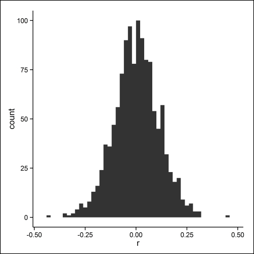
Figure 4.5
The examples so far show how auto-encoders can be trained, but have only represented shallow auto-encoders with a single hidden layer. We can also have deep auto-encoders with multiple hidden layers.
Given that we know the MNIST dataset consists of 10 different handwritten digits, perhaps we might try adding a second layer of hidden neurons with only 10 neurons, supposing that, when the model learns the features of the data, 10 prominent features may correspond to the 10 digits.
To add this second layer of hidden neurons, we pass a vector, c(100, 10), to the hidden argument, and update the hidden_dropout_ratios argument as well, because a different dropout ratio can be used for each hidden layer:
m3 <- h2o.deeplearning(
  x = xnames,
  training_frame= h2odigits.train,
  validation_frame = h2odigits.test,
  activation = "Tanh",
  autoencoder = TRUE,
  hidden = c(100, 10),
  epochs = 30,
  sparsity_beta = 0,
  input_dropout_ratio = 0,
  hidden_dropout_ratios = c(0, 0),
  l1 = 0,
  l2 = 0
)
As we saw previously, we can extract the values for the hidden neurons. Here we again use the h2o.deepfeatures() function, but we specify that we want the values for layer 2. The first six rows of these features are shown next:
features3 <- as.data.frame(h2o.deepfeatures(m3, h2odigits.train, 2))
head(features3)

  DF.L2.C1 DF.L2.C2 DF.L2.C3 DF.L2.C4 DF.L2.C5 DF.L2.C6 DF.L2.C7
1    -0.16     0.01     0.61    0.610   0.7468     0.11  -0.3927
2    -0.28    -0.77    -0.82    0.563  -0.4422    -0.66   0.6042
3    -0.48    -0.23     0.24   -0.141   0.3252     0.42  -0.0088
4    -0.30    -0.37     0.42   -0.313   0.1896    -0.27   0.1442
5    -0.36    -0.73    -0.84    0.733  -0.4807    -0.62   0.6828
6    -0.24     0.16    -0.10   -0.037  -0.0064    -0.20   0.4794
  DF.L2.C8 DF.L2.C9 DF.L2.C10
1    0.023    -0.39     0.385
2    0.321    -0.39    -0.079
3    0.589     0.59     0.538
4   -0.224    -0.31     0.557
5    0.347    -0.62    -0.098
6   -0.592     0.11     0.253
Because there are no outcomes being predicted, these values are continuous and are not probabilities of there being a particular digit, but just values on 10 continuous hidden neurons.
Next we can add in the actual digit labels from the training data, and use the melt() function to reshape the data into a long dataset. From there, we can plot the means on each of the 10 hidden layers by which digit a case actually belongs to. If the 10 hidden features roughly correspond to the 10 digit labels, for particular labels (for example, 0, 3, etc.) they should have an extreme value on one deep feature, indicating the correspondence between a deep feature and the actual digits. The results are shown in Figure 4.6:
features3$label <- digits.train$label[i]
features3 <- melt(features3, id.vars = "label")

p.line <- ggplot(features3, aes(as.numeric(variable), value,
                      colour = label, linetype = label)) +
  stat_summary(fun.y = mean, geom = "line") +
  scale_x_continuous("Deep Features", breaks = 1:10) +
  theme_classic() +
  theme(legend.position = "bottom", legend.key.width = unit(1, "cm"))
print(p.line)
Figure 4.6
Although there does seem to be some correspondence (for example, zeros are particularly high on deep features 4 and 7), in general the results are quite noisy without particularly clear indication of a high degree of separation between deep features and the actual digit labels.
Finally, we can take a look at the performance metrics for the model. With an MSE of about 0.039, the model fits substantially worse than did the shallow model, probably because having only 10 hidden neurons for the second layer is too simplistic to capture all the different features of the data needed to reproduce the original inputs:
m3
Training Set Metrics:
=====================

MSE: (Extract with `h2o.mse`) 0.039

H2OAutoEncoderMetrics: deeplearning
** Reported on validation data. **

Validation Set Metrics:
=====================

MSE: (Extract with `h2o.mse`) 0.04
This section has shown the basics of training an auto-encoder model, the code, and some ways of evaluating its performance. In the next section, we will examine a use case: finding anomalous values using an auto-encoder.