
In this chapter we will explore how to train and build deep prediction models. We will focus on feedforward neural networks, which are perhaps the most common type and a good starting point.
This chapter will cover the following topics:
- Getting started with deep feedforward neural networks
- Common activation functions: rectifiers, hyperbolic tangent, and maxout
- Picking hyperparameters
- Training and predicting new data from a deep neural network
- Use case – training a deep neural network for automatic classification
In this chapter, we will not use any new packages. The only requirements are to source the checkpoint.R file to set up the R environment for the rest of the code shown and to initialize the H2O cluster. Both can be done using the following code:
source("checkpoint.R")
options(width = 70, digits = 2)

cl <- h2o.init(
  max_mem_size = "12G",
nthreads = 4)A deep feedforward neural network is designed to approximate a function, f(), that maps some set of input variables, x, to an output variable, y. They are called feedforward neural networks because information flows from the inputs through each successive layer as far as the output, and there are no feedback or recursive loops (models including both forward and backward connections are referred to as recurrent neural networks).
Deep feedforward neural networks are applicable to a wide range of problems, and are particularly useful for applications such as image classification. More generally, feedforward neural networks are useful for prediction and classification where there is a clearly defined outcome (what digit an image contains, whether someone is walking upstairs or walking on a flat surface, the presence/absence of disease, and so on). In these cases, there is no particular need for a feedback loop. Recurrent networks are useful for cases where feedback loops are important, such as for natural language processing. However, these are outside the scope of this book, which will focus on training standard prediction models.
Deep feedforward neural networks can be constructed by chaining layers or functions together. For example, a network with four hidden layers is shown in Figure 5.1:
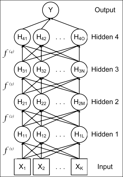
Figure 5.1
A different function is learned for each successive layer, and to finally map the hidden layers to the outcome. If sufficient hidden neurons are included in a layer, it can approximate to the desired degree of precision with many different types of functions. Even if the mapping from the final hidden layer to the outcome is a linear mapping with learned weights, feedforward neural networks can approximate non-linear functions, by first applying non-linear transformations from the input layer to the hidden layer. This is one of the key strengths of deep learning. In linear regression, for example, the model learns the weights from the inputs to the outcome. However, the functional form must be specified. In deep feedforward neural networks, the transformations from the input layer to the hidden layer are learned as well as the weights from the hidden layer to the outcome. In essence, the model learns the functional form as well as the weights. In practice, although it is unlikely that the model will learn the true generative model, it can (closely) approximate the true model. The more hidden neurons, the closer the approximation. Thus for practical, if not theoretically exact, purposes, the model learns the functional form.
Figure 5.1 shows a diagram of the model as a directed acyclic graph. Represented as a function, the overall mapping from the inputs, X, to the output, Y, is a multi-layered function. The first hidden layer is H1 = f(1)(X, w1, α1), the second hidden layer is H2 = f(2)(H1, w2, α2), and so on. These multiple layers can allow complex functions and transformations to be built up from relatively simple ones.
The weights for each layer will be learned by the machine, but are also dependent on decisions made, such as how many hidden neurons should be in each layer and the activation function to be used, a topic explored further in the next section. Another key piece of the model that must be determined is the cost or loss function. The two most commonly used cost functions are cross-entropy and mean squared error (MSE), which is quadratic.