In order to run this app (chapter7.py), we need to set up a screen capture by using cv2.VideoCapture and pass the handle to the FaceLayout class:

import time
import wx
from os import path
import cPickle as pickle

import cv2
import numpy as np

from datasets import homebrew
from detectors import FaceDetector
from classifiers import MultiLayerPerceptron
from gui import BaseLayout


def main():
    capture = cv2.VideoCapture(0)
    if not(capture.isOpened()):
        capture.open()

    capture.set(cv2.cv.CV_CAP_PROP_FRAME_WIDTH, 640)
    capture.set(cv2.cv.CV_CAP_PROP_FRAME_HEIGHT, 480)

    # start graphical user interface
    app = wx.App()
    layout = FaceLayout(None, -1, 'Facial Expression Recognition', capture)
    layout.init_algorithm()
    layout.Show(True)
    app.MainLoop()

if __name__ == '__main__':
    main()

Analogous to the previous chapters, the GUI of the app is a customized version of the generic BaseLayout:

class FaceLayout(BaseLayout):

We initialize the training samples and labels as empty lists, and make sure to call the _on_exit method upon closing the window so that the training data is dumped to file:

    def _init_custom_layout(self):
        # initialize data structure
        self.samples = []
        self.labels = []

        # call method to save data upon exiting
        self.Bind(wx.EVT_CLOSE, self._on_exit)

We also have to load several classifiers to make the preprocessing and (later on) the real-time classification work. For convenience, default file names are provided:

    def init_algorithm(
        self, save_training_file='datasets/faces_training.pkl',load_preprocessed_data='datasets/faces_preprocessed.pkl',load_mlp='params/mlp.xml',
        face_casc='params/haarcascade_frontalface_default.xml',left_eye_casc='params/haarcascade_lefteye_2splits.xml',right_eye_casc='params/haarcascade_righteye_2splits.xml'):

Here, save_training_file indicates the name of a pickle file in which to store all training samples after data acquisition is complete:

        self.dataFile = save_training_file

The three cascades are passed to the FaceDetector class as explained in the previous section:

        self.faces = FaceDetector(face_casc, left_eye_casc, right_eye_casc)

As their names suggest, the remaining two arguments (load_preprocessed_data and load_mlp) are concerned with a real-time classification of the detected faces by using the pre-trained MLP classifier:

        # load preprocessed dataset to access labels and PCA 
        # params
        if path.isfile(load_preprocessed_data):
            (_, y_train), (_, y_test), self.pca_V, self.pca_m =homebrew.load_from_file(load_preprocessed_data)
            self.all_labels = np.unique(np.hstack((y_train, 
                y_test)))

            # load pre-trained multi-layer perceptron
            if path.isfile(load_mlp):
                self.MLP = MultiLayerPerceptron( np.array([self.pca_V.shape[1], len(self.all_labels)]), self.all_labels)
                self.MLP.load(load_mlp)

If any of the parts required for the testing mode are missing, we print a warning and disable the testing mode altogether:

            else:
                print "Warning: Testing is disabled"
                print "Could not find pre-trained MLP file ", 
                    load_mlp
                self.testing.Disable()
        else:
            print "Warning: Testing is disabled"
            print "Could not find preprocessed data file ", loadPreprocessedData
        self.testing.Disable()

Creation of the layout is again deferred to a method called _create_custom_layout. We keep the layout as simple as possible: We create a panel for the acquired video frame, and draw a row of buttons below it.

The idea is to then click one of the six radio buttons to indicate which facial expression you are trying to record, then place your head within the bounding box, and click the Take Snapshot button.

Below the current camera frame, we place two radio buttons to select either the training or the testing mode, and tell the GUI that the two are mutually exclusive by specifying style=wx.RB_GROUP:

def _create_custom_layout(self):
    # create horizontal layout with train/test buttons
    pnl1 = wx.Panel(self, -1)
    self.training = wx.RadioButton(pnl1, -1, 'Train', (10, 10), style=wx.RB_GROUP)
    self.testing = wx.RadioButton(pnl1, -1, 'Test')
    hbox1 = wx.BoxSizer(wx.HORIZONTAL)
    hbox1.Add(self.training, 1)
    hbox1.Add(self.testing, 1)
    pnl1.SetSizer(hbox1)

Also, we want the event of a button click to bind to the self._on_training and self._on_testing methods, respectively:

self.Bind(wx.EVT_RADIOBUTTON, self._on_training, self.training)
self.Bind(wx.EVT_RADIOBUTTON, self._on_testing, self.testing)

The second row should contain similar arrangements for the six facial expression buttons:

# create a horizontal layout with all buttons
pnl2 = wx.Panel(self, -1 )
self.neutral = wx.RadioButton(pnl2, -1, 'neutral', (10, 10), style=wx.RB_GROUP)
self.happy = wx.RadioButton(pnl2, -1, 'happy')
self.sad = wx.RadioButton(pnl2, -1, 'sad')
self.surprised = wx.RadioButton(pnl2, -1, 'surprised')
self.angry = wx.RadioButton(pnl2, -1, 'angry')
self.disgusted = wx.RadioButton(pnl2, -1, 'disgusted')
hbox2 = wx.BoxSizer(wx.HORIZONTAL)
hbox2.Add(self.neutral, 1)
hbox2.Add(self.happy, 1)

hbox2.Add(self.sad, 1)
hbox2.Add(self.surprised, 1)
hbox2.Add(self.angry, 1)
hbox2.Add(self.disgusted, 1)
pnl2.SetSizer(hbox2)

The Take Snapshot button is placed below the radio buttons and will bind to the _on_snapshot method:

pnl3 = wx.Panel(self, -1)
self.snapshot = wx.Button(pnl3, -1, 'Take Snapshot')
self.Bind(wx.EVT_BUTTON, self.OnSnapshot, self.snapshot)
hbox3 = wx.BoxSizer(wx.HORIZONTAL)
hbox3.Add(self.snapshot, 1)
pnl3.SetSizer(hbox3)

This will look like the following:

To make these changes take effect, the created panels need to be added to the list of existing panels:

# display the button layout beneath the video stream
self.panels_vertical.Add (pnl1, flag=wx.EXPAND | wx.TOP, border=1)
self.panels_vertical.Add(pnl2, flag=wx.EXPAND | wx.BOTTOM, border=1)
self.panels_vertical.Add(pnl3, flag=wx.EXPAND | wx.BOTTOM, border=1)

The rest of the visualization pipeline is handled by the BaseLayout class. Now, whenever the user clicks the self.testing button, we no longer want to record training samples, but instead switch to the testing mode. In the testing mode, none of the training-related buttons should be enabled, as shown in the following image:

This can be achieved with the following method that disables all the relevant buttons:

def _on_testing(self, evt):
    """Whenever testing mode is selected, disable all training-related buttons"""
    self.neutral.Disable()
    self.happy.Disable()
    self.sad.Disable()
    self.surprised.Disable()
    self.angry.Disable()
    self.disgusted.Disable()
    self.snapshot.Disable()

Analogously, when we switch back to the training mode, the buttons should be enabled again:

def _on_training(self, evt):
    """Whenever training mode is selected, enable all 
        training-related buttons"""
    self.neutral.Enable()
    self.happy.Enable()
    self.sad.Enable()
    self.surprised.Enable()
    self.angry.Enable()
    self.disgusted.Enable()
    self.snapshot.Enable()

The rest of the visualization pipeline is handled by the BaseLayout class. We only need to make sure to provide the _process_frame method. This method begins by detecting faces in a downscaled grayscale version of the current frame, as explained in the previous section:

def _process_frame(self, frame):
    success, frame, self.head = self.faces.detect(frame)

If a face is found, success is True, and the method has access to an annotated version of the current frame (frame) and the extracted head region (self.head). Note that we store the extracted head region for further reference, so that we can access it in _on_snapshot.

We will return to this method when we talk about the testing mode, but for now, this is all we need to know. Don't forget to pass the processed frame:

    return frame

When the Take Snapshot button is clicked upon, the _on_snapshot method is called. This method detects the emotional expression that we are trying to record by checking the value of all radio buttons, and assigns a class label accordingly:

def _on_snapshot(self, evt):
    if self.neutral.GetValue():
        label = 'neutral'
    elif self.happy.GetValue():
        label = 'happy'
    elif self.sad.GetValue():
        label = 'sad'
    elif self.surprised.GetValue():
        label = 'surprised'
    elif self.angry.GetValue():
        label = 'angry'
    elif self.disgusted.GetValue():
        label = 'disgusted'

We next need to look at the detected facial region of the current frame (stored in self.head by _process_frame), and align it with all the other collected frames. That is, we want all the faces to be upright and the eyes to be aligned. Otherwise, if we do not align the data samples, we run the risk of having the classifier compare eyes to noses. Because this computation can be costly, we do not apply it on every frame, but instead only upon taking a snapshot. The alignment takes place in the following method:

    if self.head is None:
        print "No face detected"
    else:
        success, head = self.faces.align_head(self.head)

If this method returns True for success, indicating that the sample was successfully aligned with all other samples, we add the sample to our dataset:

if success:
    print "Added sample to training set"
    self.samples.append(head.flatten())
    self.labels.append(label)
else:
    print "Could not align head (eye detection failed?)"

All that is left to do now is to make sure that we save the training set upon exiting.

Upon exiting the app (for example, by clicking the Close button of the window), an event EVT_CLOSE is triggered, which binds to the _on_exit method. This method simply dumps the collected samples and the corresponding class labels to file:

def _on_exit(self, evt):
    """Called whenever window is closed"""
    # if we have collected some samples, dump them to file
    if len(self.samples) > 0:

However, we want to make sure that we do not accidentally overwrite previously stored training sets. If the provided filename already exists, we append a suffix and save the data to the new filename instead:

    # make sure we don't overwrite an existing file
    if path.isfile(self.data_file):
        filename, fileext = path.splitext(self.data_file)
        offset = 0
        while True: # a do while loop
            file = filename + "-" + str(offset) + fileext
            if path.isfile(file):
                offset += 1
            else:
                break
        self.data_file = file

Once we have created an unused filename, we dump the data to file by making use of the pickle module:

    f = open(self.dataFile, 'wb')
    pickle.dump(self.samples, f)
    pickle.dump(self.labels, f)
    f.close()

Upon exiting, we inform the user that a file was created and make sure that all data structures are correctly deallocated:

    print "Saved", len(self.samples), "samples to", self.data_file
    self.Destroy()

Here are some examples from the assembled training set I:

Analogous to Chapter 6, Learning to Recognize Traffic Signs, we write a new dataset parser in dataset/homebrew.py that will parse our self-assembled training set. We define a load_data function that will parse the dataset, perform feature extraction, split the data into training and testing sets, and return the results:

import cv2
import numpy as np

import csv
from matplotlib import cm
from matplotlib import pyplot as plt

from os import path
import cPickle as pickle


def load_data(load_from_file, test_split=0.2, num_components=50, 
    save_to_file=None, plot_samples=False, seed=113):
    """load dataset from pickle """

Here, load_from_file specifies the path to the data file that we created in the previous section. We can also specify another file called save_to_file, which will contain the dataset after feature extraction. This will be helpful later on when we perform real-time classification.

The first step is thus to try and open load_from_file. If the file exists, we use the pickle module to load the samples and labels data structures; else, we throw an error:

# prepare lists for samples and labels
X = []
labels = []
if not path.isfile(load_from_file):
    print "Could not find file", load_from_file
    return (X, labels), (X, labels), None, None
else:
    print "Loading data from", load_from_file
    f = open(load_from_file, 'rb')
    samples = pickle.load(f)
    labels = pickle.load(f)
    print "Loaded", len(samples), "training samples"

If the file was successfully loaded, we perform PCA on all samples. The num_components variable specifies the number of principal components that we want to consider. The function also returns a list of basis vectors (V) and a mean value (m) for every sample in the set:

# perform feature extraction
# returns preprocessed samples, PCA basis vectors & mean
X, V, m = extract_features(samples, num_components=num_components)

As pointed out earlier, it is imperative to keep the samples that we use to train our classifier separate from the samples that we use to test it. For this, we shuffle the data and split it into two separate sets, such that the training set contains a fraction (1 - test_split) of all samples, and the rest of the samples belong to the test set:

# shuffle dataset
np.random.seed(seed)
np.random.shuffle(X)
np.random.seed(seed)
np.random.shuffle(labels)

# split data according to test_split
X_train = X[:int(len(X)*(1-test_split))]
y_train = labels[:int(len(X)*(1-test_split))]

X_test = X[int(len(X)*(1-test_split)):]
y_test = labels[int(len(X)*(1-test_split)):]

If specified, we want to save the preprocessed data to file:

if save_to_file is not None:
    # dump all relevant data structures to file
    f = open(save_to_file, 'wb')
    pickle.dump(X_train, f)
    pickle.dump(y_train, f)
    pickle.dump(X_test, f)
    pickle.dump(y_test, f)
    pickle.dump(V, f)
    pickle.dump(m, f)
    f.close()
    print "Save preprocessed data to", save_to_file

Finally, we can return the extracted data:

return (X_train, y_train), (X_test, y_test), V, m

PCA is a dimensionality reduction technique that is helpful whenever we are dealing with high-dimensional data. In a sense, you can think of an image as a point in a high-dimensional space. If we flatten a 2D image of height m and width n (by concatenating either all rows or all columns), we get a (feature) vector of length m × n. The value of the i-th element in this vector is the grayscale value of the i-th pixel in the image. To describe every possible 2D grayscale image with these exact dimensions, we will need an m × n dimensional vector space that contains 256 raised to the power of m × n vectors. Wow! An interesting question that comes to mind when considering these numbers is as follows: could there be a smaller, more compact vector space (using less than m × n features) that describes all these images equally well? After all, we have previously realized that grayscale values are not the most informative measures of content.

This is where PCA comes in. Consider a dataset from which we extracted exactly two features. These features could be the grayscale values of pixels at some x and y positions, but they could also be more complex than that. If we plot the dataset along these two feature axes, the data might lie within some multivariate Gaussian, as shown in the following image:

What PCA does is rotate all data points until the data lie aligned with the two axes (the two inset vectors) that explain most of the spread of the data. PCA considers these two axes to be the most informative, because if you walk along them, you can see most of the data points separated. In more technical terms, PCA aims to transform the data to a new coordinate system by means of an orthogonal linear transformation. The new coordinate system is chosen such that if you project the data onto these new axes, the first coordinate (called the first principal component) observes the greatest variance. In the preceding image, the small vectors drawn correspond to the eigenvectors of the covariance matrix, shifted so that their tails come to lie at the mean of the distribution.

Fortunately, someone else has already figured out how to do all this in Python. In OpenCV, performing PCA is as simple as calling cv2.PCACompute. Embedded in our feature extraction method, the option reads as follows:

def extract_feature(X, V=None, m=None, num_components=50):

Here, the function can be used to either perform PCA from scratch or use a previously calculated set of basis vectors (V) and mean (m), which is helpful during testing when we want to perform real-time classification. The number of principal components to consider is specified via num_components. If we do not specify any of the optional arguments, PCA is performed from scratch on all the data samples in X:

    if V is None or m is None:
        # need to perform PCA from scratch
        if num_components is None:
            num_components = 50
 
        # cols are pixels, rows are frames
        Xarr = np.squeeze(np.array(X).astype(np.float32))

        # perform PCA, returns mean and basis vectors
        m, V = cv2.PCACompute(Xarr)

The beauty of PCA is that the first principal component by definition explains most of the variance of the data. In other words, the first principal component is the most informative of the data. This means that we do not need to keep all of the components to get a good representation of the data! We can limit ourselves to the num_components most informative ones:

    # use only the first num_components principal components
    V = V[:num_components]

Finally, a compressed representation of the data is achieved by projecting the zero-centered original data onto the new coordinate system:

    for i in xrange(len(X)):
        X[i] = np.dot(V, X[i] - m[0, i])

    return X, V, m

A perceptron is a binary classifier that was invented in the 1950s by Frank Rosenblatt. A perceptron calculates a weighted sum of its inputs, and if this sum exceeds a threshold, it outputs a 1; else, it outputs a 0. In some sense, a perceptron is integrating evidence that its afferents signal the presence (or absence) of some object instance, and if this evidence is strong enough, the perceptron will be active (or silent). This is loosely connected to what researchers believe biological neurons are doing (or can be used to do) in the brain, hence, the term artificial neural network.

A sketch of a perceptron is depicted in the following figure:

Here, a perceptron computes a weighted (w_i) sum of all its inputs (x_i), combined with a bias term (b). This input is fed into a nonlinear activation function (θ) that determines the output of the perceptron (y). In the original algorithm, the activation function was the Heaviside step function. In modern implementations of ANNs, the activation function can be anything ranging from sigmoid to hyperbolic tangent functions. The Heaviside function and the sigmoid function are plotted in the following image:

Depending on the activation function, these networks might be able to perform either classification or regression. Traditionally, one only talks of MLPs when nodes use the Heaviside step function.

Once you have the perceptron figured out, it would make sense to combine multiple perceptrons to form a larger network. Multi-layer perceptrons usually consist of at least three layers, where the first layer has a node (or neuron) for every input feature of the dataset, and the last layer has a node for every class label. The layer in between is called the hidden layer. An example of this feed-forward neural network is shown in the following figure:

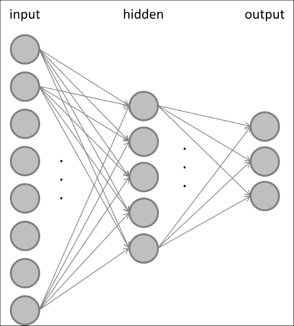
In a feed-forward neural network, some or all of the nodes in the input layer are connected to all the nodes in the hidden layer, and some or all of the nodes in the hidden layer are connected to some or all of the nodes in the output layer. You would usually choose the number of nodes in the input layer to be equal to the number of features in the dataset, so that each node represents one feature. Analogously, the number of nodes in the output layer is usually equal to the number of classes in the data, so that when an input sample of class c is presented, the c-th node in the output layer is active and all others are silent.

It is also possible to have multiple hidden layers of course. Often, it is not clear beforehand what the optimal size of the network should be.

Typically, you will see the error rate on the training set decrease when you add more neurons to the network, as is depicted in the following figure (thinner, red curve):

This is because the expressive power or complexity (also referred to as the Vapnik–Chervonenkis or VC dimension) of the model increases with the increasing size of the neural network. However, the same cannot be said for the error rate on the test set (thicker, blue curve)! Instead, what you will find is that with increasing model complexity, the test error goes through a minimum, and adding more neurons to the network will not improve the generalization performance any more. Therefore, you would want to steer the size of the neural network to what is labeled the optimal range in the preceding figure, which is where the network achieves the best generalization performance.

You can think of it this way. A model of weak complexity (on the far left of the plot) is probably too small to really understand the dataset that it is trying to learn, thus yielding large error rates on both the training and the test sets. This is commonly referred to as underfitting. On the other hand, a model on the far right of the plot is probably so complex that it begins to memorize the specifics of each sample in the training data, without paying attention to the general attributes that make a sample stand apart from the others. Therefore, the model will fail when it has to predict data that it is has never seen before, effectively yielding a large error rate on the test set. This is commonly referred to as overfitting.

Instead, what you want is to develop a model that neither underfits nor overfits. Often this can only be achieved by trial-and-error; that is, by considering the network size as a hyperparameter that needs to be tweaked and tuned depending on the exact task to be performed.

An MLP learns by adjusting its weights so that when an input sample of class c is presented, the c-th node in the output layer is active and all the others are silent. MLPs are trained by means of backpropagation, which is an algorithm to calculate the partial derivative of a loss function with respect to any synaptic weight or neuron bias in the network. These partial derivatives can then be used to update the weights and biases in the network in order to reduce the overall loss step-by-step.

A loss function can be obtained by presenting training samples to the network and by observing the network's output. By observing which output nodes are active and which are silent, we can calculate the relative error between what the output layer is doing and what it should be doing (that is, the loss function). We then make corrections to all the weights in the network so that the error decreases over time. It turns out that the error in the hidden layer depends on the output layer, and the error in the input layer depends on the error in both the hidden layer and the output layer. Thus, in a sense, the error (back)propagates through the network. In OpenCV, backpropagation is used by specifying cv3.ANN_MLP_TRAIN_PARAMS_BACKPROP in the training parameters.

Following the requirements defined by the Classifier base class, we need to perform training in a fit method:

def fit(self, X_train, y_train, params=None):
    """ fit model to data """
    if params is None:
        params = self.params

Here, params is an optional dictionary that contains a number of options relevant to training, such as the termination criteria (term_crit) and the learning algorithm (train_method) to be used during training. For example, to use backpropagation and terminate training either after 300 iterations or when the loss reaches values smaller than 0.01, specify params as follows:

params = dict(
    term_crit = (cv2.TERM_CRITERIA_COUNT, 300, 0.01), train_method = cv2.ANN_MLP_TRAIN_PARAMS_BACKPROP)

Because the train method of the cv2.ANN_MLP module does not allow integer-valued class labels, we need to first convert y_train into "one-hot" code, consisting only of zeros and ones, which can then be fed to the train method:

y_train = self._labels_str_to_num(y_train)
y_train = self._one_hot(y_train).reshape(-1, self.num_classes)
    self.model.train(X_train, y_train, None, params=params)

The one-hot code is taken care of in _one_hot:

def _one_hot(self, y_train):
    """Convert a list of labels into one-hot code """

Each class label c in y_train needs to be converted into a self.num_classes-long vector of zeros and ones, where all entries are zeros except the c-th, which is a one. We prepare this operation by allocating a vector of zeros:

    num_samples = len(y_train)
    new_responses = np.zeros(num_samples * self.num_classes, np.float32)

Then, we identify the indices of the vector that correspond to all the c-th class labels:

    resp_idx = np.int32(y_train + 
        np.arange(num_samples)  self.num_classes)

The vector elements at these indices then need to be set to one:

    new_responses[resp_idx] = 1
    return new_responses

Following the requirements defined by the Classifier base class, we need to perform training in an evaluate method:

def evaluate(self, X_test, y_test, visualize=False):
    """ evaluate model performance """

Analogous to the previous chapter, we will evaluate the performance of our classifier in terms of accuracy, precision, and recall. To reuse our previous code, we again need to come up with a 2D voting matrix, where each row stands for a data sample in the testing set and the c-th column contains the number of votes for the c-th class.

In the world of perceptrons, the voting matrix actually has a straightforward interpretation: The higher the activity of the c-th neuron in the output layer, the stronger the vote for the c-th class. So, all we need to do is to read out the activity of the output layer and plug it into our accuracy method:

    ret, Y_vote = self.model.predict(X_test)
    y_test = self._labels_str_to_num(y_test)
    accuracy = self._accuracy(y_test, Y_vote)
    precision = self._precision(y_test, Y_vote)
    recall = self._recall(y_test, Y_vote)

    return (accuracy, precision, recall)

In addition, we expose the predict method to the user, so that it is possible to predict the label of even a single data sample. This will be helpful when we perform real-time classification, where we do not want to iterate over all test samples, but instead only consider the current frame. This method simply predicts the label of an arbitrary number of samples and returns the class label as a human-readable string:

def predict(self, X_test):
    """ predict the labels of test data """
    ret, Y_vote = self.model.predict(X_test)

    # find the most active cell in the output layer
    y_hat = np.argmax(Y_vote, 1)

    # return string labels
    return self._labels_num_to_str(y_hat)

The MLP classifier can be trained and tested by using the train_test_mlp.py script. The script first parses the homebrew dataset and extracts all class labels:

import cv2
import numpy as np

from datasets import homebrew
from classifiers import MultiLayerPerceptron

def main():
    # load training data
    # training data can be recorded using chapter7.py in training 
    # mode
    (X_train, y_train),(X_test, y_test) =
        homebrew.load_data("datasets/faces_training.pkl", num_components=50, test_split=0.2, save_to_file="datasets/faces_preprocessed.pkl", seed=42)
    if len(X_train) == 0 or len(X_test) == 0:
        print "Empty data"
    raise SystemExit

    # convert to numpy
    X_train = np.squeeze(np.array(X_train)).astype(np.float32)
    y_train = np.array(y_train)
    X_test = np.squeeze(np.array(X_test)).astype(np.float32)
    y_test = np.array(y_test)

    # find all class labels
    labels = np.unique(np.hstack((y_train, y_test)))

We also make sure to provide some valid termination criteria as described above:

    params = dict( term_crit = (cv2.TERM_CRITERIA_COUNT, 300, 0.01), train_method=cv2.ANN_MLP_TRAIN_PARAMS_BACKPROP, bp_dw_scale=0.001, bp_moment_scale=0.9 )

Often, the optimal size of the neural network is not known a priori, but instead, a hyperparameter needs to be tuned. In the end, we want the network that gives us the best generalization performance (that is, the network with the best accuracy measure on the test set). Since we do not know the answer, we will run a number of different-sized MLPs in a loop and store the best in a file called saveFile:

    save_file = 'params/mlp.xml'
    num_features = len(X_train[0])
    num_classes = len(labels)

    # find best MLP configuration
    print "1-hidden layer networks"
    best_acc = 0.0 # keep track of best accuracy
    for l1 in xrange(10):
        # gradually increase the hidden-layer size
        layer_sizes = np.int32([num_features, 
            (l1 + 1) * num_features / 5, 
            num_classes])
    MLP = MultiLayerPerceptron(layer_sizes, labels)
    print layer_sizes

The MLP is trained on X_train and tested on X_test:

    MLP.fit(X_train, y_train, params=params)
    (acc, _, _) = MLP.evaluate(X_train, y_train)
    print " - train acc = ", acc
    (acc, _, _) = MLP.evaluate(X_test, y_test)
    print " - test acc = ", acc

Finally, the best MLP is saved to file:

    if acc > best_acc:
        # save best MLP configuration to file
        MLP.save(saveFile)
    best_acc = acc

The saved params/mlp.xml file that contains the network configuration and learned weights can then be loaded into the main GUI application (chapter7.py) by passing loadMLP='params/mlp.xml' to the init_algorithm method of the FaceLayout class. The default arguments throughout this chapter will make sure that everything works straight out of the box.