As we saw in the last chapter, a fast and robust way of extracting important features from an image is by using a SURF detector. In this chapter, we want to use it for two images, self.img1 and self.img2:

def _extract_keypoints_surf(self):
    detector = cv2.SURF(250)
    first_key_points, first_des = detector.detectAndCompute(self.img1, None)
    second_key_points, second_desc = detector.detectAndCompute(self.img2, None)

For feature matching, we will use a BruteForce matcher, but other matchers (such as FLANN) can work as well:

matcher = cv2.BFMatcher(cv2.NORM_L1, True)
matches = matcher.match(first_desc, second_desc)

For each of the matches, we need to recover the corresponding image coordinates. These are maintained in the self.match_pts1 and self.match_pts2 lists:

first_match_points = np.zeros((len(matches), 2), dtype=np.float32)
second_match_points = np.zeros_like(first_match_points)
for i in range(len(matches)):
    first_match_points[i] = 
        first_key_points[matches[i].queryIdx].pt
    second_match_points[i] = 
        second_key_points[matches[i].trainIdx].pt

self.match_pts1 = first_match_points
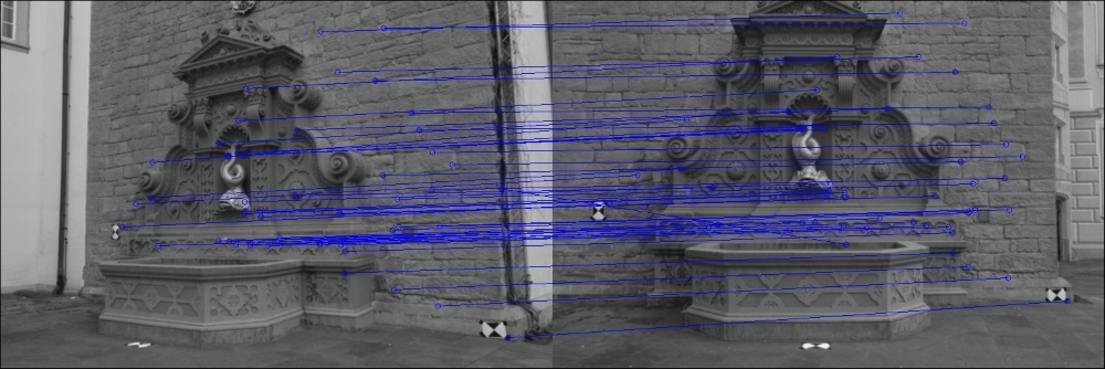
self.match_pts2 = second_match_points

The following screenshot shows an example of the feature matcher applied to two arbitrary frames of the fountain sequence:

An alternative to using rich features, is using optic flow. Optic flow is the process of estimating motion between two consecutive image frames by calculating a displacement vector. A displacement vector can be calculated for every pixel in the image (dense) or only for selected points (sparse).

One of the most commonly used techniques for calculating dense optic flow is the Lukas-Kanade method. It can be implemented in OpenCV with a single line of code, by using the cv2.calcOpticalFlowPyrLK function.

But before that, we need to select some points in the image that are worth tracking. Again, this is a question of feature selection. If we were interested in getting an exact result for only a few highly salient image points, we can use Shi-Tomasi's cv2.goodFeaturesToTrack function. This function might recover features like this:

However, in order to infer structure from motion, we might need many more features and not just the most salient Harris corners. An alternative would be to detect the FAST features:

def _extract_keypoints_flow(self):
    fast = cv2.FastFeatureDetector()
    first_key_points = fast.detect(self.img1, None)

We can then calculate the optic flow for these features. In other words, we want to find the points in the second image that most likely correspond to the first_key_points from the first image. For this, we need to convert the keypoint list into a NumPy array of (x,y) coordinates:

first_key_list = [i.pt for i in first_key_points]
first_key_arr = np.array(first_key_list).astype(np.float32)

Then the optic flow will return a list of corresponding features in the second image (second_key_arr):

second_key_arr, status, err = cv2.calcOpticalFlowPyrLK(self.img1, self.img2, first_key_arr)

The function also returns a vector of status bits (status), which indicate whether the flow for a keypoint has been found or not, and a vector of estimated error values (err). If we were to ignore these two additional vectors, the recovered flow field could look something like this:

In this image, an arrow is drawn for each keypoint, starting at the image location of the keypoint in the first image and pointing to the image location of the same keypoint in the second image. By inspecting the flow image, we can see that the camera moved mostly to the right, but there also seems to be a rotational component. However, some of these arrows are really large, and some of them make no sense. For example, it is very unlikely that a pixel in the bottom-right image corner actually moved all the way to the top of the image. It is much more likely that the flow calculation for this particular keypoint is wrong. Thus, we want to exclude all the keypoints for which the status bit is zero or the estimated error is larger than some value:

condition = (status == 1) * (err < 5.)
concat = np.concatenate((condition, condition), axis=1)
first_match_points = first_key_arr[concat].reshape(-1, 2)
second_match_points = second_key_arr[concat].reshape(-1, 2)

self.match_pts1 = first_match_points
self.match_pts2 = second_match_points

If we draw the flow field again with a limited set of keypoints, the image will look like this:

The flow field can be drawn with the following public method, which first extracts the keypoints using the preceding code and then draws the actual lines on the image:

def plot_optic_flow(self):
    self._extract_key_points("flow")

    img = self.img1
    for i in xrange(len(self.match_pts1)):
        cv2.line(img, tuple(self.match_pts1[i]), tuple(self.match_pts2[i]), color=(255, 0, 0))
        theta = np.arctan2(self.match_pts2[i][1] – self.match_pts1[i][1], self.match_pts2[i][0] – self.match_pts1[i][0])
        cv2.line(img, tuple(self.match_pts2[i]),
             (np.int(self.match_pts2[i][0] – 6*np.cos(theta+np.pi/4)),
             np.int(self.match_pts2[i][1] – 
             6*np.sin(theta+np.pi/4))), color=(255, 0, 0))
        cv2.line(img, tuple(self.match_pts2[i]), (np.int(self.match_pts2[i][0] –6*np.cos(theta-np.pi/4)),np.int(self.match_pts2[i][1] – 
            6*np.sin(theta-np.pi/4))), color=(255, 0, 0))
    for i in xrange(len(self.match_pts1)):
        cv2.line(img, tuple(self.match_pts1[i]), tuple(self.match_pts2[i]), color=(255, 0, 0))
        theta = np.arctan2(self.match_pts2[i][1] -self.match_pts1[i][1],self.match_pts2[i][0] - self.match_pts1[i][0])
    cv2.imshow("imgFlow",img)
    cv2.waitKey()

The advantage of using optic flow instead of rich features is that the process is usually faster and can accommodate the matching of many more points, making the reconstruction denser.

The caveat in working with optic flow is that it works best for consecutive images taken by the same hardware, whereas rich features are mostly agnostic to this.

Now that we have obtained the matches between keypoints, we can calculate two important camera matrices: the fundamental matrix and the essential matrix. These matrices will specify the camera motion in terms of rotational and translational components. Obtaining the fundamental matrix (self.F) is another OpenCV one-liner:

def _find_fundamental_matrix(self):
    self.F, self.Fmask = cv2.findFundamentalMat(self.match_pts1, self.match_pts2, cv2.FM_RANSAC, 0.1, 0.99)

The only difference between the fundamental matrix and the essential matrix is that the latter operates on rectified images:

def _find_essential_matrix(self):
    self.E = self.K.T.dot(self.F).dot(self.K)

The essential matrix (self.E) can then be decomposed into rotational and translational components, denoted as [R | t], using singular value decomposition (SVD):

def _find_camera_matrices(self):
    U, S, Vt = np.linalg.svd(self.E)
    W = np.array([0.0, -1.0, 0.0, 1.0, 0.0, 0.0, 0.0, 0.0, 1.0]).reshape(3, 3)

Using the unitary matrices U and V in combination with an additional matrix, W, we can now reconstruct [R | t]. However, it can be shown that this decomposition has four possible solutions and only one of them is the valid second camera matrix. The only thing we can do is check all four possible solutions and find the one that predicts that all the imaged keypoints lie in front of both cameras.

But prior to that, we need to convert the keypoints from 2D image coordinates to homogeneous coordinates. We achieve this by adding a z coordinate, which we set to 1:

first_inliers = []
second_inliers = []
for i in range(len(self.Fmask)):
    if self.Fmask[i]:
        first_inliers.append(self.K_inv.dot([self.match_pts1[i][0], self.match_pts1[i][1], 1.0]))
        second_inliers.append(self.K_inv.dot([self.match_pts2[i][0], self.match_pts2[i][1], 1.0]))

We then iterate over the four possible solutions and choose the one that has _in_front_of_both_cameras returning True:

# First choice: R = U * Wt * Vt, T = +u_3 (See Hartley 
# & Zisserman 9.19)
R = U.dot(W).dot(Vt)
T = U[:, 2]

if not self._in_front_of_both_cameras(first_inliers,second_inliers, R, T):
    # Second choice: R = U * W * Vt, T = -u_3
    T = - U[:, 2]

if not self._in_front_of_both_cameras(first_inliers, second_inliers, R, T):
    # Third choice: R = U * Wt * Vt, T = u_3
    R = U.dot(W.T).dot(Vt)
    T = U[:, 2]

if not self._in_front_of_both_cameras(first_inliers, second_inliers, R, T):
    # Fourth choice: R = U * Wt * Vt, T = -u_3
    T = - U[:, 2]

Now, we can finally construct the [R | t] matrices of the two cameras. The first camera is simply a canonical camera (no translation and no rotation):

self.Rt1 = np.hstack((np.eye(3), np.zeros((3, 1))))

The second camera matrix consists of [R | t] recovered earlier:

self.Rt2 = np.hstack((R, T.reshape(3, 1)))

The __InFrontOfBothCameras private method is a helper function that makes sure that every pair of keypoints is mapped to 3D coordinates that make them lie in front of both cameras:

def _in_front_of_both_cameras(self, first_points, second_points, rot, trans):
    rot_inv = rot
    for first, second in zip(first_points, second_points):
        first_z = np.dot(rot[0, :] - second[0]*rot[2, :], trans) / np.dot(rot[0, :] - second[0]*rot[2, :], second)
        first_3d_point = np.array([first[0] * first_z, second[0] * first_z, first_z])
        second_3d_point = np.dot(rot.T, first_3d_point) – np.dot(rot.T, trans)

If the function finds any keypoint that is not in front of both cameras, it will return False:

if first_3d_point[2] < 0 or second_3d_point[2] < 0:
    return False
return True

Maybe, the easiest way to make sure that we have recovered the correct camera matrices is to rectify the images. If they are rectified correctly, then; a point in the first image, and a point in the second image that correspond to the same 3D world point, will lie on the same vertical coordinate. In a more concrete example, such as in our case, since we know that the cameras are upright, we can verify that horizontal lines in the rectified image correspond to horizontal lines in the 3D scene.

First, we perform all the steps described in the previous subsections to obtain the [R | t] matrix of the second camera:

def plot_rectified_images(self, feat_mode="SURF"):
    self._extract_keypoints(feat_mode)
    self._find_fundamental_matrix()
    self._find_essential_matrix()
    self._find_camera_matrices_rt()

    R = self.Rt2[:, :3]
    T = self.Rt2[:, 3]

Then, rectification can be performed with two OpenCV one-liners that remap the image coordinates to the rectified coordinates based on the camera matrix (self.K), the distortion coefficients (self.d), the rotational component of the essential matrix (R), and the translational component of the essential matrix (T):

    R1, R2, P1, P2, Q, roi1, roi2 = cv2.stereoRectify(self.K, self.d, self.K, self.d, self.img1.shape[:2], R, T,
        alpha=1.0)
    mapx1, mapy1 = cv2.initUndistortRectifyMap(self.K, self.d, R1, self.K, self.img1.shape[:2], cv2.CV_32F)
    mapx2, mapy2 = cv2.initUndistortRectifyMap(self.K, self.d, R2, self.K, self.img2.shape[:2], cv2.CV_32F)
    img_rect1 = cv2.remap(self.img1, mapx1, mapy1, cv2.INTER_LINEAR)
    img_rect2 = cv2.remap(self.img2, mapx2, mapy2, cv2.INTER_LINEAR)

To make sure that the rectification is accurate, we plot the two rectified images (img_rect1 and img_rect2) next to each other:

total_size = (max(img_rect1.shape[0], img_rect2.shape[0]), img_rect1.shape[1] + img_rect2.shape[1], 3)
img = np.zeros(total_size, dtype=np.uint8)
img[:img_rect1.shape[0], :img_rect1.shape[1]] = img_rect1
img[:img_rect2.shape[0], img_rect1.shape[1]:] = img_rect2

We also draw horizontal blue lines after every 25 pixels, across the side-by-side images to further help us visually investigate the rectification process:

for i in range(20, img.shape[0], 25):
    cv2.line(img, (0, i), (img.shape[1], i), (255, 0, 0))
    cv2.imshow('imgRectified', img)

Now we can easily convince ourselves that the rectification was successful, as shown here: