
2
MBB Service – Spatial Multiplexing
2.1. Multiplexing techniques
2.1.1. MIMO mechanism
The term SU-MIMO (Single-User Multiple Input Multiple Output) refers to a transmission to the same mobile, using the same frequency and time resource, on two antennas (MIMO 2 × 2) (Figure 2.1), four antennas (MIMO 4 × 4) or eight antennas (MIMO 8 × 8).

Figure 2.1. SU-MIMO mechanism
The term MU-MIMO (Multi-User MIMO) refers to a transmission to different mobiles, using the same frequency and time resource, on two antennas (MIMO 2 × 2) (Figure 2.2), four antennas (MIMO 4 × 4) or eight antennas (MIMO 8 × 8).

Figure 2.2. MU-MIMO mechanism
The MIMO mechanism improves the radio interface data rate thanks to the spatial multiplexing transmission of different signals emitted by the different antennas, each transmission sharing the same frequency and time resource.
The signal x1 (respectively x2) is transmitted by the transmitter Tx1 (respectively Tx2). The signal y1 (respectively y2) is received by the receiver Rx1 (respectively Rx2). The transmission matrix H contains the transfer functions hij, from the transmitter j to the receiver i.
On the reception side, the received signals y1 and y2 are the product of the transmitted signals x1 and x2 by the transmission matrix H.

The spatial demultiplexing consists of recovering the components x1 and x2 from the received signals y1 and y2 and the knowledge of the transmission matrix H.

The inverse matrix is estimated using two methods: minimum mean square error (MMSE) or zero forcing (ZF).
2.1.2. Beamforming
Beamforming is a complementary mechanism of MIMO. The beamforming technique uses multiple antennas to control the beam direction by individually weighting the amplitude and phase of each transmitted signal, by applying a specific precoding matrix to each component of the transmitted signal (Figure 2.3).
The precoding matrix can be determined by the mobile using the direction of arrivals (DoA). This technique is based on the analysis of the spectrum (the main lobe and the secondary lobes) of the received signal whose peaks identify the arrival angles.
Using beamforming, it is possible to logically reduce the beam opening angle and to limit the level of interference between the cells.
Using beamforming, it is also possible to increase the range thanks to the gain of power due to the contribution of each emitted signal.

Figure 2.3. Beamforming
2.1.3. Antenna configurations
The transmission modes implementing beamforming and MU-MIMO require a good correlation between the antennas.
The transmission modes implementing transmission diversity and SU-MIMO require a decorrelation between the antennas.
For an antenna made of columns of radiating components with vertical polarization, the correlation between the columns is relatively strong.
For an antenna made of a column of two sets of radiating components, each set corresponding to a crossed polarization ± 45 degrees, the correlation is relatively weak.
The antenna configurations are described in Figure 2.4 and relate to a single frequency band.
Configuration A corresponds to an antenna made of a column of radiating components with vertical polarization.
Configuration B corresponds to an antenna made of a dual column of radiating components with vertical polarization.
Configuration C corresponds to an antenna made of four columns of radiating components with vertical polarization.
Configuration D corresponds to an antenna made of a column of two sets of radiating components, each set corresponding to a crossed polarization ± 45 degrees.
Configuration E corresponds to an antenna made of two columns, each column comprising two radiating component sets, each set corresponding to a crossed polarization ± 45 degrees.
Configuration E combines pairs of correlated radiating components of the same polarization, and pairs of decorrelated radiating components with different polarization.
Configuration F corresponds to an antenna made with:
- – a central column of two sets of radiating components, each set corresponding to a crossed polarization ± 45 degrees;
- – two separate sets, each set comprising radiating components, corresponding to one of the two crossed polarizations ± 45 degrees.
The remaining polarization remains available for use in another frequency band.
Configuration G corresponds to an antenna made of four columns of radiating components, each column comprising two sets of radiating components, each set corresponding to a crossed polarization ± 45 degrees.
Configuration H corresponds to two separate antennas, each antenna being made of a column of two sets of radiating components, each set corresponding to a crossed polarization ± 45 degrees.
Configuration I corresponds to two separate antennas, each antenna being made of a column of radiating components with vertical polarization.
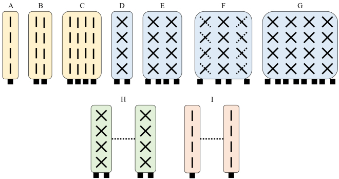
Figure 2.4. Antenna configurations
2.2. Antenna ports
2.2.1. Downlink
The symbols produced by the modulation are distributed over spatial layers, and then precoded.
The precoded symbols are associated with the reference signal (RS) to form antenna ports.
Table 2.1 shows the association of the antenna ports and the reference signals for the downlink.
Each of the antenna ports p0 to p3 is associated with a physical antenna.
The antenna port p4 is associated with a single physical antenna.
The antenna port p5 is associated with two or four physical antennas.
The antenna port p6 is associated with a single physical antenna.
Each of the antenna ports p7 to p14 and p15 to p22 is associated with a physical antenna.
Table 2.1. Association of the antenna ports and reference signals: downlink
| Antenna ports | Reference signal |
| p0 to p3 | CRS |
| p4 | MBSFN-RS |
| p5 | UE-specific RS |
| p6 | PRS |
| p7 and p8 | UE-specific RS |
| p9 to p14 | UE-specific RS |
| p15 to p22 | CSI-RS |
2.2.1.1. CRS
The cell-specific reference signal (CRS) is used to perform coherent demodulation of the received signal.
The coherent demodulation of the received signal is based on the calculation of the transfer function of the radio channel.
The CRS allows the implementation of spatial multiplexing and transmission diversity.
The CRS makes it possible to measure the reference signal received power (RSRP) and the reference signal received quality (RSRQ).
The CRS is transmitted in each sub-frame and covers the entire bandwidth of the radio channel.
2.2.1.2. MBSFN-RS
The MBMS single frequency network reference signal (MBSFN-RS) is only transmitted in the physical multicast channel (PMCH) for coherent demodulation of the received signal.
The PMCH is used to transmit IP (Internet Protocol) packets in the broadcast mode.
2.2.1.3. UE-specific RS
The UE-specific reference signal is used for the beamforming mechanism and for the spatial multiplexing of multiple users, and allows the demodulation of the physical downlink shared channel (PDSCH).
The UE-specific RS allows the following configurations:
- – one user using a single spatial layer;
- – one user using two spatial layers, and a beamforming associated with MIMO 2 × 2;
- – two users using two spatial layers, the multiplexing of the two users being carried out by an identity code;
- – four users using a spatial layer, the multiplexing of the four spatial layers being obtained from an orthogonal covering code (OCC) and an identity code;
- – one user using eight spatial layers, and a beamforming associated with the MIMO 8 × 8.
2.2.1.4. PRS
The positioning reference signal (PRS) is used by the mobile to implement the observed time difference of arrival (OTDOA).
The OTDOA function is based on the measurement by the mobile of the difference in the time of reception of the PRS with respect to a reference cell.
The location of the mobile is obtained from three measurements made on three geographically dispersed cells.
2.2.1.5. CSI-RS
The channel state information reference signal (CSI-RS) improves the measurement of the received signal and the level of interference compared to that provided from the CRS-RS.
The power of the CSI-RS is either transmitted to determine the level of the received signal or suppressed to measure the level of interference.
2.2.2. Uplink
Table 2.2 shows the association of the antenna ports and the physical channels or signals for the uplink.
The number of the antenna port depends on the number of antenna ports identified by the index ![]() .
.
Table 2.2. Numbering of antenna ports for the uplink
| Physical channel or signal | Index |
Antenna ports | ||
| 1 port | 2 ports | 4 ports | ||
| PUSCH SRS | 0 | 10 | 20 | 40 |
| 1 | – | 21 | 41 | |
| 2 | – | – | 42 | |
| 3 | – | – | 43 | |
| PUCCH | 0 | 100 | 200 | – |
| 1 | – | 201 | – | |
Antenna ports 10 and 100 use a single physical antenna ![]()
Antenna ports 20 and 200 (21 and 201 respectively) use the physical antenna ![]() respectively).
respectively).
Each of the antenna ports 40 to 43 uses a physical antenna.
2.3. UCI
The uplink control information (UCI) is information transmitted by the mobile and contains the scheduling request (SR), the HARQ indicator (HI) and the CSI.
The HI relates the positive (ACK) or negative (NACK) acknowledgment of data received on the PDSCH.
The CSI, estimated by the mobile, regroups the information related to the status report of the signal received on the PDSCH:
- – the channel quality indicator (CQI) represents the modulation and coding scheme recommended for the PDSCH;
- – the rank indicator (RI) determines the number of spatial layers recommended for the PDSCH;
- – the precoder matrix indicator (PMI) provides indications related to the precoding matrix in the case of using spatial multiplexing, in closed loop, or in the case of beamforming.
The report of the CSI can be periodic or aperiodic.
The aperiodic report is always transferred in the physical uplink shared channel (PUSCH).
The periodic report is transferred in the physical uplink control channel (PUCCH) in the two following cases:
- – no resource is allocated to the mobile in the PUSCH;
- – a resource is allocated to the mobile and the simultaneous transmission of the PUCCH and PUSCH is possible.
Otherwise, the periodic report is transmitted in the PUSCH.
The report transfer modes are built based on the return type of CQI and PMI.
The type of transfer of the aperiodic or periodic report is communicated to the mobile by the RRC (Radio Resource Control) messages: ConnectionSetup, ConnectionReconfiguration or ConnectionReconfiguration.
The aperiodic report allows feedback related to the CSI in relation to the totality or to a part of the bandwidth of the radio channel defined by the mobile or the eNB entity (Table 2.3).
The transfer of the aperiodic report is triggered by the following messages:
- – the downlink control information (DCI) transmitted in the physical downlink control channel (PDCCH);
- – the random access response (RAR) transmitted in the PDSCH.
The periodic report allows feedback to the CSI in relation to the totality or to a part of the bandwidth of the radio channel defined only by the eNB entity (Table 2.4).
Table 2.3. Transfer modes of the aperiodic reports
| Return PMI | ||||
| No PMI | Single PMI | Multiple PMI | ||
| CQI return | Wide band | Mode 1-2 | ||
| Sub-band per UE | Mode 2-0 | Mode 2-2 | ||
| Sub-band per eNB | Mode 3-0 | Mode 3-1 | ||
Table 2.4. Transfer modes of the periodic reports
| Return PMI | |||
| No PMI | Single PMI | ||
| CQI return | Wide band | Mode 1-0 | Mode 1-1 |
| Sub-band per eNB | Mode 2-0 | Mode 2-1 | |
2.4. Transmission modes
2.4.1. Downlink
Transmission mode 1 (TM1) is the SISO (Single Input Single Output) type. It corresponds to setting a transmitter to the antenna port p0. When the mobile is equipped with two receptors, it can implement the reception diversity.
Transmission mode 2 (TM2) is specified for MISO (Multiple Input Single Output). It corresponds to setting several transmitters of the same signal to the antenna ports p0 and p1 in the case of two transmitters, or p0 to p3 in the case of four transmitters to support the transmission diversity which facilitates the improvement of the quality of the received signal.
In the case of transmission using two antenna ports p0 and p1, the transmission diversity corresponds to the space-frequency block coding (SFBC). In the case of transmission using four antenna ports p0 to p3, the transmission diversity corresponds to the SFBC/FSTD (Frequency Shift Transmit Diversity) mechanism.
Transmission mode 3 (TM3) is specified for open-loop SU-MIMO. It corresponds to setting two transmitters of different signals and two receivers (SU-MIMO 2 × 2) using the antenna ports p0 and p1, or four transmitters and four receivers (SU-MIMO 4 × 4) using the antenna ports p0 to p3.
TM3 supports the spatial multiplexing function with an open-loop control which facilitates the improvement of the throughput of the cell.
TM3 uses a precoding matrix with cyclic delay diversity (CDD). The CDD method consists of applying a fixed precoding, the possible values of which are defined in a codebook.
Transmission mode 4 (TM4) is specified for closed-loop SU-MIMO. It corresponds to setting two transmitters of different signals and two receivers (SU-MIMO 2 × 2) using the antenna ports p0 and p1, or four transmitters and four receivers (SU-MIMO 4 × 4) using the antenna ports p0 to p3.
TM4 supports the spatial multiplexing function in a closed loop. The mobile transmits in the PMI the pre-encoding index selected in the codebook.
Transmission mode 5 (TM5) is specified for MU-MIMO. It supports the spatial multiplexing function with a closed-loop control, for two users (MU-MIMO 2 × 2) or four users (MU-MIMO 4 × 4).
Transmission mode 6 (TM6) corresponds to a simplified version of TM4, for which a single spatial layer is used.
Transmission mode 7 (TM7) supports the beamforming function. This mode uses the antenna port p5.
TM7 can also simultaneously support the MU-MIMO function, for providing spatial multiplexing of several users in an open loop, with each user granted one layer.
TM7 is suitable for the time-division duplex (TDD), for which the sharing between the transmission for the upstream and downstream directions takes place temporally.
Transmission mode 8 (TM8) is an extension of TM7. The spatial multiplexing allows the following configurations:
- – two users with an allocation of two spatial layers per user;
- – four users with an allocation of one spatial layer per user.
TM8 uses the antenna ports p7 and p8.
Transmission mode 9 (TM9) is configured either for SU-MIMO 8 × 8, for beamforming or for MU-MIMO. TM9 is associated with the antenna ports p7 to p14.
Transmission mode 10 (TM10) is similar to TM9. The main difference comes from CoMP (Coordinated Multi Point) transmission, for which the transmitting antennas can be physically located on different sites.
Table 2.5 summarizes the various modes of transmission, the evolved node base station (eNB) being able to switch between several transmission modes.
Table 2.5. Downlink transmission modes
| Mode | Transmission scheme |
| 1 | SISO, antenna port p0 |
| 2 | Transmit diversity (MISO) |
| 3 | Transmit diversity (MISO) |
| SU-MIMO, open loop | |
| 4 | Transmit diversity (MISO) |
| SU-MIMO, closed loop | |
| 5 | Transmit diversity (MISO) |
| MU-MIMO | |
| 6 | Transmit diversity (MISO) |
| SU-MIMO, closed loop one spatial layer | |
| 7 | Transmit diversity (MISO) or SISO, antenna port p0 |
| Beamforming and MU-MIMO antenna port p5 | |
| 8 | Transmit diversity (MISO) or SISO, antenna port p0 |
| Beamforming and MU-MIMO antenna ports p7 and p8 | |
| 9 | Transmit diversity (MISO) or SISO, antenna port p0 |
| Beamforming and MU-MIMO antenna ports p7 to p14 | |
| 10 | Transmit diversity (MISO) or SISO, antenna port p0 |
| Beamforming and MU-MIMO antenna ports p7 to p14 CoMP |
The correspondence between the antenna configuration, described in section 2.3, and the transmission modes is given in Table 2.6.
Table 2.6. Correspondence between the configuration of the antennas and modes of transmission
| Antenna configuration | Transmission modes |
| A | TM1 |
| B | TM5, TM7 for TDD |
| C | TM5, TM7 to TM8 for TDD |
| D | TM2 to TM4, TM6 |
| E | TM2 to TM6, TM7 to TM8 for TDD |
| F | TM2 to TM6 |
| G | TM2 to TM6, TM7 to TM8 for TDD, TM9 |
| H | TM2 to TM6 |
| I | TM2 to TM4, TM6 |
2.4.2. Uplink
Since the mobile is equipped with two antennas, the transmission can be carried out on one of the two antennas; the selection of the antenna is performed either by the mobile or by the eNB entity. If the eNB entity is equipped with two receptors, it can implement the reception diversity.
Transmission mode 1 (TM1) is the SISO type. It corresponds to setting a transmitter to the antenna port p10 for the PUSCH or to the antenna port p100 for the PUCCH.
Transmission mode 2 (TM2) is the MIMO type for the PUSCH. It corresponds to setting two transmitters of different signals on the antenna ports p20 and p21 (MIMO 2 × 2) or four transmitters on the antenna ports p40 to p43 (MIMO 4 × 4) to support the spatial multiplexing in a closed loop.
TM2 uses transmit diversity for the PUCCH. It corresponds to setting two transmitters of the same signal on the antenna ports p200 and p201.
2.5. FD-MIMO mechanism
The elevation beamforming (EBF) allows a beam to be directed in a specific manner, for example a beam pointing either to the top or to the bottom. This technique contrasts with conventional antennal systems for which the tilt angle is fixed.
The FD-MIMO (Full-Dimension MIMO) mechanism is based on the elevation beamforming in the vertical plane and in the horizontal plane (Figure 2.5). Both directions can be combined, leading to two-dimensional beamforming.

Figure 2.5. Beamforming in different planes
(source: NTT DOCOMO Technical Reports Journal, vol. 18 no. 2)
This new beamforming technique tends to increase the number of antennas since the signal has spatial access to more degrees of freedom. It is implemented by an active antenna system (AAS).
The AAS consists of a block of TXU transmitters and TRU receivers, a radio distribution network (RDN) and an antenna array (AA) (Figure 2.6).

Figure 2.6. AAS
The transmitter block TXU takes the baseband signals delivered by the common public radio interface (CPRI) and outputs the radio frequency signals. Each baseband signal can be assigned to one or more TXU transmitters. The RF outputs are distributed to the antenna array via the radio distribution network (RDN). The receiver block TRU performs the reverse operation.
In order to provide an elevation of a zenith angle θetilt, the RDN weights the radio frequency signal supplied by the unit TXU by a coefficient w. The same operation is performed for the signal received from the antenna array.
The configuration of an antenna array is given by the parameters (M, N and P), where M is the number of antenna elements having the same polarization in each column (M = {1, 2, 4, 8}), N is the number of columns (N = {1, 2, 4, 8, 16}) and P is the number of polarizations (normally equal to 2).
MTXRU is the number of TXU/TRU per column and polarization and NTXRU is the number of TXU/TRU per row and polarization.
Two generic models of mapping between the antenna elements {M, N, P} and the TXU/TRU {MTXRU, NTXRU} have been defined: the sub-array partition model and the full-connection model.
For the sub-array partition model (Figure 2.7), the antenna elements are distributed among different groups and each TXU/TRU is connected to a group. The weighting value wk of the radio signal is provided by the following formula:

where:

- λ is the wavelength;
- dv is the distance separating two antenna elements vertically;
- θetilt is the zenith angle.
For the full-connection model (Figure 2.7), each TXU/TRU is connected to each antenna element. A combiner is used to couple the different TXU/TRU on each antenna element. The value of the weighting wm,m’ of the radio signal is provided by the following formula:


Figure 2.7. Mapping between the TXU/TRU and the antenna elements
The main changes in FD-MIMO compared to traditional MIMO are given in Table 2.7.
Table 2.7. Comparison between MIMO and FD-MIMO
| Mechanism | MIMO | FD-MIMO |
| Number of antenna ports CSI-RS | 1, 2, 4, 8 | 1, 2, 4, 8, 12, 16 |
| Beamforming | Horizontal plane | Horizontal and vertical planes |
| Number of radio signal SU-MIMO | 8 | 8 |
| Number of radio signal MU-MIMO | 4 (note 1) | 8 (note 2) |
Note 1: the maximum number of mobiles spatially multiplexed is equal to 4. The number of radio signals per mobile is then equal to 2.
Note 2: the maximum number of mobiles spatially multiplexed is equal to 8. The number of radio signals per mobile is then equal to 2.
The FD-MIMO mechanism introduces two methods for CSI feedback to the eNB entity: the Class A method and the Class B method.
The Class A method is applied to the sub-array partition model and consists of reassembling the CSI by antenna element and polarization of a group from the non-precoded CSI-RS.
The Class A method defines a number of non-precoded CSI-RS and a number of antenna ports that can vary from 1 to 16, which limits the configuration of the antenna, and adopts a codebook identical to the one defined for the transmission mode TM9, for each plane (horizontal or vertical).
The CSI-RS uses two resource elements for each antenna port. The use of the orthogonal covering code (OCC) makes it possible to consume only two resource elements for two antenna ports.
There are 40 resource elements reserved for mapping the CSI-RS:
- – in the case of eight antenna ports, the CSI-RS consumes eight resource elements. There are therefore five different configurations;
- – in the case of four antenna ports, the CSI-RS consumes four resource elements. There are therefore 10 different configurations.
Table 2.8 shows the constitution of the antenna ports to obtain the values equal to 12 and 16 from an aggregation of configurations.
Figure 2.8 shows a mapping of the CSI-RS on the resource elements, for 12 and 16 antenna ports.
Table 2.8. Constitution of the antenna ports: FD-MIMO
| Number of antenna ports | Number of antenna ports per configuration | Number of configurations |
| 12 | 4 | 3 |
| 16 | 8 | 2 |

Figure 2.8. CSI-RS mapping: FD-MIMO
The Class B method is applied to the full-connection model and consists of reporting the CSI for each beam formed from the CSI-RS.
The Class B method limits the number of CSI-RS and the number of antenna ports to 8. This number is independent of the number of antenna elements used by the radio signal.
The reported CSI relates to the best received CSI-RS and contains a CSI resource index (CRI) corresponding to this CSI-RS.
2.6. eFD-MIMO mechanism
The eFD-MIMO (enhanced FD-MIMO) mechanism provides the following enhancements to the CSI-RS:
- – increasing the number {20, 24, 28, 32} of reference signals;
- – reducing the overhead introduced by the reference signals.
Table 2.9. Constitution of the antenna ports: eFD-MIMO
| Number of antenna ports | Number of antenna ports per configuration | Number of configuration |
| 20 | 4 | 5 |
| 24 | 8 | 3 |
| 28 | 4 | 7 |
| 32 | 8 | 4 |
Table 2.9 shows the constitution of the antenna ports to obtain the values between 20 and 32 from an aggregation of configurations.
Figure 2.9 shows a mapping of the CSI-RS on the resource elements, for 20 and 32 antenna ports. The overhead is equal to 11.9% (respectively 19%) for a number of CSI-RS equal to 20 (respectively 32).
Reducing the overhead consists of configuring the frequency density of the CSI-RS with a normal density of value 1 or with a reduced density of value {1/2, 1/3}.

Figure 2.9. CSI-RS reference signal mapping: eFD-MIMO
The reduction of the overhead is achieved by transmitting the CSI-RS in one pair of resource blocks in two (density 1/2) or in three (density 1/3).
For the Class B method, the following mechanisms have been introduced to allow more efficient use of CSI-RS resources formed by a mobile-specific beam, for example, to enable more mobile to share a CSI-RS resource pool:
- – aperiodic CSI-RS, wherein a mobile is configured to measure the CSI-RS in a given sub-frame;
- – multi-shot CSI-RS, wherein a mobile is configured to measure the periodic CSI-RS for a determined period of time.
Two-step resource configurations, combining the use of RRC messages and MAC (Medium Access Control) elements, are introduced to allow flexible selection of resources while maintaining control over CSI reporting overhead.
The improvements also include the optimization of CSI reports obtained from CSI-RS measurements.
The first mechanism aims to improve the quality of CSI feedback by adopting a two-step CSI report. In the first step, CSI reporting is obtained from a non-precoded physical signal measurement (Class A method). In the second step, CSI reporting is obtained from a measurement of the CSI-RS formed by a beam (Class B method).
The second mechanism aims to provide greater flexibility in the use of CSI-RS resources with a limited number of CSI processes. CSI reporting is realized with one CSI process (Class B method) with K>1 CSI-RS resources for the first step and with K=1 CSI-RS resources for the second step.