
6
Predicting the Risk of Gestational Diabetes Mellitus through Nearest Neighbor Classification
Gestational diabetes mellitus (GDM) may arise as a complication of pregnancy and can adversely affect both mother and child. Diagnosis of this condition is carried out through screening coupled with an oral glucose test. This procedure is costly and time-consuming. Therefore, it would be desirable if a clinical risk assessment method could filter out any individuals who are not at risk of acquiring this disease. This problem can be tackled as a binary classification problem. In this study, our aim is to compare and contrast the results obtained through binary logistic regression (BLR), used in previous studies, and three well-known non-parametric classification techniques, namely the k-nearest neighbors (kNN) method, the fixed-radius-NN method and the kernel-NN method. These techniques were selected due to their relative simplicity, applicability, lack of assumptions and nice theoretical properties. The test dataset contains information related to 1,368 subjects across 11 Mediterranean countries. Using various performance measures, the results revealed that NN methods succeeded in outperforming the BLR method.
6.1. Introduction
The World Health Organization (WHO) defines diabetes mellitus as “a chronic, metabolic disease characterized by elevated levels of blood glucose (or blood sugar), which leads over time to serious damage to the heart, blood vessels, eyes, kidneys and nerves”. Gestational diabetes mellitus (GDM) is a form of diabetes which arises as a complication of pregnancy. Alfadhli (2015) discusses how, worldwide, the prevalence of this disease fluctuates between 1% and 20%, and these rates are higher for certain ethnic groups such as Indian, African, Hispanic and Asian women. In 2010, the International Association of Diabetes and Pregnancy Study Group (IADPSG) established new criteria for the diagnosis of GDM; pregnant women are screened, and the oral glucose tolerance test (OGTT) is used for diagnosis.
Savona-Ventura et al. (2013) explained that the screening, as well as the OGTT, are costly diagnostic methods. To this end, an alternative clinical risk assessment method for GDM, based on explanatory variables that can be easily measured at minimal cost, is sought to preclude these tests, especially in countries and health centers dealing with budget cuts and a lack of resources. The prediction of the risk of an individual acquiring GDM is a problem that can be tackled using a variety of classification techniques. Savona-Ventura et al. (2013) applied binary logistic regression (BLR). In the literature, some shortcomings of the BLR model devised in the study by Savona-Ventura et al. (2013) are outlined. Kotzaeridi et al. (2021) remark that this model tended to underestimate the risk of GDM. Furthermore, Lamain-de Ruiter et al. (2017) found that this same model also involved a moderate risk of bias when compared to other models. Thus, we seek alternative methods which may serve as an improvement over the BLR model implemented by Savona-Ventura et al. (2013). Nearest neighbor (NN) methods, which are non-parametric classification techniques, were found to be commonly used in studies involving the prediction of diabetes mellitus. Kandhasamy and Balamuali (2015) compared the performance of four popular classification techniques, namely the J48 decision tree, the k-nearest neighbor (kNN) classifier, random forests and support vector machines (SVMs), in predicting the risk of diabetes mellitus for noisy (or inconsistent) data with missing values and for consistent data. The study showed that the J48 decision tree performed best for the noisy data, while random forests and the kNN classifier with k = 1 performed best for the consistent data. Furthermore, Saxena et al. (2004) discuss in detail the use of kNN in classifying diabetes mellitus. The authors applied this algorithm to a dataset consisting of 11 variables, among which were glucose concentration, age, sex and body mass index. Saxena et al. (2004) then analyzed the results obtained for k = 3 and k = 5 through the use of well-known performance measures; the results of the study led to the conclusion that the error rate increased for the larger value of k, and so better results were obtained for k = 3.
In this chapter, our main aim is to test the applicability and the performance of three well-known NN methods, to the problem of predicting the risk of GDM. In particular, we focus on the application of the kNN method, the fixed-radius-NN method and the kernel-NN method. These methods will be applied to a dataset pertaining to 1,368 pregnant women from 11 Mediterranean countries. More specifically, the dataset consists of 71 explanatory variables such as age, pre-existing hypertension, menstrual cycle regularity and history of diabetes in the family. Since the classification accuracy may be affected by factors such as the presence of missing data or an imbalance between the considered classes, imputation techniques will be implemented to deal with missing values, while the class imbalance between the positive and negative cases for GDM will be tackled through a technique called SMOTE-NC. The performance of these methods will then be evaluated and compared through the use of various performance measures. In addition, the results obtained will be compared to those obtained in Savona-Ventura et al. (2013), where BLR has been applied to the same dataset.
The rest of this chapter is structured as follows. In section 6.2, we discuss in detail the NN techniques used in this chapter, as well as presenting some important convergence results. In section 6.3, we provide a thorough description of the dataset used and the corresponding preliminary data analysis; we also present and compare the results obtained from the implementation of NN methods and BLR. Finally, section 6.4 contains the concluding remarks of this study.
6.2. Nearest neighbor methods
6.2.1. Background of the NN methods
We begin this section by introducing some notations that will be used throughout this chapter. The problem being tackled here involves binary prediction, which means having two possible class labels: positive for GDM (1) and negative for GDM (0). Thus, let Y be a random variable that represents a possible class label of an individual, and let X = (X1,... , Xp) be a p-dimensional random vector whose components, which are random variables, represent a certain feature in the dataset, for example, the age of the mother and number of miscarriages. Also, let x = (x1,..., xp) be a vector of observed values. In a classification problem, we make use of a dataset comprising a finite sample of independent, identically distributed pairs (x1, y1),..., (xn, yn), where yi indicates the class label of the ith observation, for i = 1,..., n, and n denotes the sample size. Then, we aim at using this dataset to estimate a function ![]() that, given a newly obtained observation/feature vector x, outputs a predicted label
that, given a newly obtained observation/feature vector x, outputs a predicted label ![]() . The function
. The function ![]() is called a classifier. The best classifier in terms of minimizing probability of error is the so-called Bayes classifier and is defined as follows:
is called a classifier. The best classifier in terms of minimizing probability of error is the so-called Bayes classifier and is defined as follows:
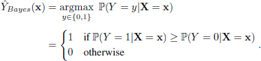
In words, the Bayes classifier compares the conditional probabilities ℙ(Y = 0|X = x) and ℙ(Y = 1|X = x), given the observed feature vector X = x and if the former is higher than the latter, it predicts x to have label 0, otherwise it predicts x to have label 1. By defining η(x) = ℙ(Y = 1|X = x), it can easily be shown that equation [6.1] can be re-written as follows:
It was shown by Chen and Shah (2018) that the Bayes classifier in equation [6.2] is indeed the one that minimizes the probability of a misclassification. Thus, any classification procedure cannot do better than the Bayes classifier. Unfortunately, in classification, we do not know the Bayes classifier ![]() and have to estimate it from training data. In the next sections, we will see how we can define/approximate the function η using three different NN methods.
and have to estimate it from training data. In the next sections, we will see how we can define/approximate the function η using three different NN methods.
6.2.2. The k-nearest neighbors method
The kNN algorithm is a non-parametric method that is used for classification and regression. In the former, to decide the class label of a feature vector, we consider the k points in the set of observed data that are closest to the point of interest. An object is allocated to the most common class among its k nearest neighbors, where k ∈ ℤ+ and usually takes on a small value. If k = 1, then the object is merely predicted to belong to the same class as that single nearest neighbor.
Using the set-up shown in the previous section, we now proceed to define an estimate ![]() for η(x)= ℙ(Y = 1|X = x) as follows:
for η(x)= ℙ(Y = 1|X = x) as follows:
where Y(i) = 1 if the ith neighbor of x has label 1 and 0 otherwise. Hence, an estimate for equation [6.2] is as follows:
Over the years, a number of results concerning upper and lower bounds on misclassification errors of the kNN classifier as well as a number of convergence guarantees have been proven. These can be found in Chaudhuri and Dasgupta (2014). We now move on to discuss the fixed-radius NN method.
6.2.3. The fixed-radius NN method
The fixed-radius NN classification method is another technique that is used in tackling binary classification problems. This method is similar to kNN, however instead of determining the test point’s label by looking at its k nearest neighbors, this point is assigned a class label through a majority vote of its neighbors that are captured within a ball of radius r. We have to note here that if the radius r, which can take any positive value, is not chosen carefully, then there is a risk of not finding any points in the neighborhood of the test point.
According to the background presented in section 2.1, an estimate ![]() for η(x) = ℙ(Y = 1|X = x), when considering the fixed-radius NN, is derived as follows:
for η(x) = ℙ(Y = 1|X = x), when considering the fixed-radius NN, is derived as follows:
where ρ represents the considered distance function and 1{·} is an indicator function taking the value of 1 if its argument is true and 0 otherwise. The difference between equations [6.5] and [6.3] is that instead of taking the average of the labels of the k-nearest neighbors of the test point, ![]() is estimated by taking the average of the labels of all points within distance r from the reference point x. Hence, an estimate of equation [6.2] is obtained by replacing η with equation [6.5] in equation [6.2] and we obtain:
is estimated by taking the average of the labels of all points within distance r from the reference point x. Hence, an estimate of equation [6.2] is obtained by replacing η with equation [6.5] in equation [6.2] and we obtain:
Convergence results related to this method were discussed in detail in Chen and Shah (2018). Next, we proceed to discuss the kernel-NN method.
6.2.4. The kernel-NN method
The kernel method makes use of a kernel function K : ℝ+ ↦ [0, 1] which takes the normalized distance between the test point and a training point (i.e. the distance calculated using some distance metric, divided by a bandwidth parameter h), and produces a similarity score, or weight, between 0 and 1. Therefore, in this case, each training point is given a weighting depending on how far it is from the test point. The aforementioned bandwidth parameter h controls this weighting; a lower bandwidth would mean that only points very close to the test point would contribute to the weighting, meaning that points far away would contribute zero or very little weight. A higher bandwidth, on the contrary, would mean that points further away from the test point would give a slightly higher contribution. Furthermore, Chen and Shah (2018) note that the kernel function is assumed to be monotonically decreasing on the positive domain, meaning that the further away a training point is from the test point, the lower its similarity score is. Guidoum (2015) remarks that, unlike the choice of the bandwidth parameter h, the choice of the kernel function is not that crucial since, as previously mentioned, the former is the one that affects which points give the most contribution, yielding equally good results for different kernel functions.
In literature, various kernel functions have been proposed. These include the uniform, Epanenchnikov, normal, biweight and triweight kernels, among others. We invite the interested reader to refer to Scheid (2004) and Guidoum (2015) for a discussion on various types of kernels. Since the choice of the kernel function is not crucial, throughout this chapter the Epanechnikov kernel was selected. Indeed, when other kernels were selected the results did not change significantly.
As in the previous two sections, we now provide an estimate for the conditional probability η. For kernel classification, this estimator is defined as follows:
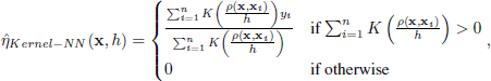
where the kernel function K determines the contribution of the ith training point to the class label prediction through a weighted average. As with the previous methods, we now replace η with ![]() in equation [6.2] to obtain the following:
in equation [6.2] to obtain the following:
Convergence results related to this method were discussed in detail in Chen and Shah (2018).
6.2.5. Algorithms of the three considered NN methods
In practice, when we want to test the classification performance of an algorithm, we need to split the available dataset of the observed feature vectors into two sets. These two sets are of unequal sizes and are called the training set and the test set; the former contains the data of m individuals, while the latter contains the data of n − m individuals. The individuals are placed in one of these two sets in a random way; however, the class proportions should be maintained to assure that the training and test sets share the same distribution characteristics. This means that if 25% of the original data belonged to the minority class, then 25% of the training set and the test set will also belong to the minority class (in our case, these are individuals that tested positive for GDM). Thus, the training set will be denoted by ((x1, y1),..., (xm, ym)) and the test set will be denoted by ((xm+1, ym+1),..., (xn, yn)). Therefore, xi, 1 ≤ i ≤ m is the feature vector that contains the observed values for the ith individual in the training set and will sometimes be called a training point. Similarly, xj, m + 1 ≤ j ≤ n is the feature vector that contains the observed values for the jth individual in the test set, and for simplicity will sometimes be called a test point. Therefore, although the class label of the test point is known, we will be using the previously described NN methods to predict it in order to evaluate the classification performance of the algorithms.
Algorithm 6.1 provides the pseudocode of kNN, while Algorithms 6.2 and 6.3 provide the pseudocode of the fixed-radius NN method and the kernel NN method, respectively.
6.2.6. Parameter and distance metric selection
The NN algorithms presented in the previous sections employ parameters that need to be appropriately selected to achieve accurate predictions. In kNN, the main parameter that needs to be appropriately selected is k, that is, the number of nearest neighbors of the test data point to be considered. Furthermore, the size of the radius r needs to be properly selected for the fixed-radius NN, while the optimal bandwidth size h needs to be selected for the kernel methods. These parameters will be selected through k-fold cross validation which in turn makes use of the maximum value of the area under the ROC curve to choose the optimal parameter.
The NN methods discussed above all require a distance metric. To this end, an appropriate distance metric must be utilized to account for the type of features in the feature space (continuous variables, categorical variables or mixed data). The choice of this metric is made particularly tricky especially in the case where a mixed dataset has to be considered; some variables are quantitative in nature, while other variables are categorical. Hence, in such cases, traditional distance metrics like the Euclidean distance are not appropriate. However, there exist distance metrics that have been designed for mixed data. These are the heterogeneous value difference metric (HVDM) and the heterogeneous Euclidean-overlap metric (HEOM) defined in Mody (2009).
In the next section, we discuss the results obtained when the above three techniques were applied to a dataset for GDM risk prediction.
6.3. Experimental results
6.3.1. Dataset description
The dataset utilized is made up of information related to 1,368 mothers and their newborn babies from 11 countries collected between 2010 and 2011. It is a mixed dataset consisting of 72 variables – 44 categorical and 28 continuous. The categorical variables also include the binary response variable that indicates whether the mother has GDM or not, thus representing the mother’s class label. We note that the number of variables in the dataset is quite large, and some may not be relevant in determining whether a mother is at risk of being diagnosed with GDM. Therefore, appropriate tests (described in section 6.3.2) were used to eliminate insignificant variables.
Furthermore, we see that 352 mothers were diagnosed with GDM according to the International Association of Diabetes and Pregnancy Study Groups’ (IADPSGs) criteria, which make up 26% of the total number of mothers. On the contrary, 1,016 mothers were found not to have GDM, making up 74% of the cases. Thus, we are dealing with imbalanced data, since the majority of mothers do not have GDM, and the minority do. This may deteriorate the performance of the classifier by increasing the false negatives. To overcome this problem, the SMOTE-NC technique as described by Chawla et al. (2002) was implemented prior to the application of the classification techniques to balance out the data.
6.3.2. Variable selection and data splitting
The robustness of NN techniques is inherently dependent on the dimension of the problem, i.e. the number of explanatory variables involved in the dataset (see Chapter 2 in Hastie et al. (2001)). High-dimensional problems favor fairly large neighborhoods of observations close to any reference point x, this way compromising the effectiveness of the estimation of ![]() in equations [6.3], [6.5] and [6.7]. Moreover, and in contrast to other parametric techniques such as BLR, all explanatory variables are equally important when NN techniques are used for making predictions, making it impossible for the algorithms themselves to identify the variables that affect the response more. Due to the reasons above, proceeding with a variable selection technique for reducing the problem’s dimension is essential.
in equations [6.3], [6.5] and [6.7]. Moreover, and in contrast to other parametric techniques such as BLR, all explanatory variables are equally important when NN techniques are used for making predictions, making it impossible for the algorithms themselves to identify the variables that affect the response more. Due to the reasons above, proceeding with a variable selection technique for reducing the problem’s dimension is essential.
In order to determine which variables are significant in diagnosing mothers with GDM, two tests were carried out at a 0.05 level of significance in accordance with the nature of each variable: a Pearson’s chi-square test for independence between GDM diagnosis and the other 43 categorical variables, and a Mann–Whitney U test between GDM diagnosis and the 28 continuous variables.
After performing a chi-square test on the categorical variables, only 12 turned out to be significant and are as follows: “Country”, “Mother’s country of birth”, “Father’s country of birth”, “Pre-existing hypertension”, “Family history: diabetes mellitus in mother”, “Family history: diabetes mellitus in father”, “Family history: diabetes mellitus in siblings”, “Menstrual cycle regularity”, “Fasting glycosuria”, “Insulin used”, “Oral medication” and “Special care baby unit admission”.
Furthermore, after implementing a Mann–Whitney U test on the continuous variables, 28 of these variables resulted as significant and were therefore retained. These include “Age”, “Pre-pregnancy body mass index”, “Systolic blood pressure”, “Diastolic blood pressure”, “Absolute hemoglobin A1c”, “Hemoglobin A1c”, “Parity”, “Personal history: macrosomia”, “Weight pre-pregnancy”, “Weight at oral glucose tolerance test”, “Body mass index at oral glucose tolerance test”, “Fasting blood glucose”, “One-hour blood glucose”, “Two-hour blood glucose”, “Area under the curve”, “Insulin level”, “Gestational age at delivery” and “Apgar score”.
Therefore, after performing variable selection, we are left with 12 categorical and 18 continuous variables, making up 30 variables in all.
The dataset was split into two non-overlapping sets: the training set and the test set. This was carried out at an 80:20 ratio, with the training set in this case being made up of 1,094 mothers, 283 (26%) of whom were diagnosed with GDM, and the test set consisting of 274 mothers, 69 (25%) of whom were diagnosed with GDM. The class imbalance in the training set was then catered for through the use of the SMOTE-NC algorithm, as explained in Chawla et al. (2002).
6.3.3. Results
Variables were first scaled and standardized before fitting any models. The optimal hyperparameter values for all three NN methods were then found using 10-fold cross validation; namely, for kNN, k = 5, for fixed-radius NN, r = 5.2 and for kernel-NN, h = 0.19.
Table 6.1. Confusion matrix for kNN on the test set (balanced case)
| Actual | ||||
| Positive | Negative | Total | ||
| Predicted | Positive | 40 | 6 | 46 |
| Negative | 29 | 199 | 228 | |
| Total | 69 | 205 | 274 | |
In the following, we will take a look at the confusion matrices obtained for each method. Table 6.1 presents the confusion matrix for kNN, Table 6.2 presents the confusion matrix for fixed-radius NN and Table 6.3 presents the confusion matrix for kernel-NN.
Table 6.2. Confusion matrix for fixed-radius NN on the test set (balanced case)
| Actual | ||||
| Positive | Negative | Total | ||
| Predicted | Positive | 2 | 0 | 2 |
| Negative | 73 | 199 | 272 | |
| Total | 75 | 199 | 274 | |
Table 6.3. Confusion matrix for the kernel-NN on the test set (balanced case)
| Actual | ||||
| Positive | Negative | Total | ||
| Predicted | Positive | 43 | 26 | 69 |
| Negative | 2 | 203 | 205 | |
| Total | 45 | 229 | 274 | |
The BLR model was implemented by Savona-Ventura et al. (2013) in order to predict the probability of developing GDM and included three binary predictors. These indicated whether fasting blood glucose (FBG) was at a level higher than 5.0 mmol/L, whether the maternal age was greater than or equal to 30 years, and whether diastolic blood pressure was greater than or equal to 80 mmHg. This particular model was first applied to the test set in both the imbalanced case (which was that examined in Savona-Ventura et al. (2013)) and balanced cases. Tables 6.4 and 6.5 present the confusion matrices obtained for BLR applied to the imbalanced and balanced datasets, respectively.
Table 6.4. Confusion matrix for BLR on the test set using the original variables (imbalanced case)
| Actual | ||||
| Positive | Negative | Total | ||
| Predicted | Positive | 42 | 6 | 48 |
| Negative | 33 | 193 | 226 | |
| Total | 75 | 199 | 274 | |
Table 6.5. Confusion matrix for BLR on the test set using the original variables (balanced case)
| Actual | ||||
| Positive | Negative | Total | ||
| Predicted | Positive | 45 | 10 | 55 |
| Negative | 24 | 195 | 219 | |
| Total | 69 | 205 | 274 | |
After checking for multicollinearity through the Spearman correlation matrix and removing any correlated predictors, another BLR model was applied to the training set, and the parsimonious model was obtained using a backward stepwise process. In this case, seven significant variables were found and retained, namely “Country”, “Family history: diabetes mellitus in mother”, “Family history: diabetes mellitus in father”, “Parity”, “Weight at oral glucose tolerance test”, “Area under the curve” and “Apgar score”. Finally, this BLR model was then applied to the test set. The confusion matrix obtained is given in Table 6.6.
Table 6.6. Confusion matrix for BLR on the test set using only the significant variables (balanced case)
| Actual | ||||
| Positive | Negative | Total | ||
| Predicted | Positive | 49 | 7 | 56 |
| Negative | 20 | 198 | 205 | |
| Total | 69 | 205 | 274 | |
We should note that for the kNN, kernel NN and BLR methods, the proportion of true predictions as can be seen in the confusion matrices were relatively higher to those for false predictions, meaning that these techniques seem to be adequate for the data. However, for the fixed-radius NN method, the confusion matrix in the balanced case showed a high proportion of true negatives (72.6%), while the proportion of true positives (0.73%) was very low relative to false predictions. This means that this method is probably not the best for the data, since it does not perform well in diagnosing mothers who have GDM.
6.3.4. A discussion and comparison of results
Table 6.7 shows an ordering of the methods according to their overall performance on the test set, from best to worst. This was based on five performance measures, namely accuracy, area under the ROC curve, precision, sensitivity and F1 score.
We see here that BLR using the original variables on the test set in the imbalanced case (which was the original case studied by Savona-Ventura et al. (2013)) was the fifth best classification technique, surpassing fixed-radius NN which had the worst overall performance. Furthermore, BLR using the original variables on the test set in the balanced case came in fourth overall. The kNN method in the balanced case had the best AUC, and the best overall performance for the NN methods followed by the kernel method. Finally, the binary logistic regression technique applied to the balanced data after obtaining the parsimonious model performed slightly better than the kNN method and proved to perform the best overall for this dataset.
Table 6.7. Classification techniques in order of performance
| Technique | Case | Accuracy | AUC | Precision | Sensitivity | F1 Score |
| BLR | Balanced - Selected Variables | 0.902 | 0.838 | 0.875 | 0.710 | 0.784 |
| kNN | Balanced | 0.872 | 0.945 | 0.870 | 0.580 | 0.696 |
| Kernel-NN | Balanced | 0.898 | 0.913 | 0.623 | 0.956 | 0.754 |
| BLR | Balanced - Original Variables | 0.876 | 0.802 | 0.818 | 0.652 | 0.726 |
| BLR | Imbalanced - Original Variables | 0.858 | 0.765 | 0.875 | 0.560 | 0.683 |
| FR-NN | Balanced | 0.733 | 0.762 | 1.000 | 0.027 | 0.052 |
6.4. Conclusion
In this chapter, three NN techniques were studied, namely kNN, fixed-radius NN and the kernel method, and their implementation in binary classification. Upon applying these methods to the dataset, together with binary logistic regression, we conclude that in comparison to the NN methods, the binary logistic regression technique using the variables in the parsimonious model for the balanced case gave a slightly better performance; however, kNN and the kernel method performed better in relation to the binary logistic regression model applied by Savona-Ventura et al. (2013).
While carrying out this study, a limitation encountered was that 10-fold cross validation to determine the optimal hyperparameters for kNN and fixed-radius NN in Python was not computationally efficient, meaning that it took a very long time to train the algorithms. A possible improvement to the study may be the exploration of Bayesian neural networks for classification problems, where cross validation is no longer needed and so the algorithm is trained more efficiently using MCMC methods. Alternative classification methods found in the literature can also be applied and compared with NN methods to obtain the best model for prediction, namely decision trees, random forests and support vector machines, for example, which are also widely used in these types of problems.
6.5. References
Alfadhli, E.M. (2015). Gestational diabetes mellitus. Saudi Medical Journal, 36(4), 399–406.
Chaudhuri, K. and Dasgupta, S. (2014). Rates of convergence for nearest neighbour classification. Proceedings of the 27th International Conference on Neural Information Processing Systems – Volume 2, 3437–3445, Montreal.
Chawla, N.V., Bowyer, K., Hall, L.O., Kegelmeyer, W. P. (2002). SMOTE: Synthetic minority over-sampling technique. Journal of Artificial Intelligence Research, 16(1), 321–357.
Chen, G.H. and Shah, D. (2018). Explaining the success of nearest neighbour methods in prediction. Foundations and Trends in Machine Learning, 10(5–6), 337–588.
Guidoum, A.C. (2015). Kernel estimator and bandwidth selection for density and its derivatives [Online]. Available at: https://cran.r-project.org/web/packages/kedd/vignettes/kedd.pdf.
Hastie, T., Tibshirani, R., Friedman, J. (2001). The Elements of Statistical Learning: Data Mining, Inference and Prediction. Springer, New York.
Kandhasamy, J.P. and Balamuali, S. (2015). Performance analysis of classifier models to predict diabetes mellitus. Procedia Computer Science, 47, 45–51.
Kotzaeridi, G., Blatter, J., Eppel, D., Rosicky, I., Mittlboeck, M., Yerlikaya-Schatten, G., Schatten, C. (2021). Performance of early risk assessment tools to predict the later development of gestational diabetes. European Journal of Clinical Investigation, 51(23).
Lamain-de Ruiter, M., Kwee, A., Naaktgeboren, C.A., Franx, A., Moons, K., Koster, M. (2017). Prediction models for the risk of gestational diabetes: A systematic review. Diagnostic and Prognostic Research, 1, 3.
Mody, R. (2009). Optimizing the distance function for nearest neighbors classifcation. Thesis, University of California San Diego [Online]. Available at: https://escholarship.org/uc/item/9b3839xn.
Savona-Ventura, C., Vassallo, J., Marre, M., Karamanos, B.G. (2013). A composite risk assessment model to screen for gestational diabetes meillitus among Mediterranean women. International Journal of Gynecology and Obstetrics, 120(3), 240–244.
Saxena, K., Khan, D.Z., Singh, S. (2004). Diagnosis of diabetes mellitus using K nearest neighbor algorithm. International Journal of Computer Science Trends and Technology, 2(4), 36–43.
Scheid, S. (2004). Introduction to kernel smoothing [Online]. Available at: https://compdiag.molgen.mpg.de/docs/talk_05_01_04_stefanie.pdf.
Chapter written by Louisa TESTA, Mark A. CARUANA, Maria KONTORINAKI and Charles SAVONA-VENTURA.