
8
The State of the Art in Flexible Regression Models for Univariate Bounded Responses
Modeling bounded continuous responses, such as proportions and rates, is a relevant problem in methodological and applied statistics. A further issue is observed if the response takes values at the boundary of the support. Given that standard models are unsuitable, a successful and relatively recent branch of research favors modeling the response variable according to distributions that are well-defined on the restricted support. A popular and well-researched choice is the beta regression model and its augmented version. More flexible alternatives than the beta regression model, among which are the flexible beta and the variance inflated beta, have been tailored for data with outlying observations, latent structures and heavy tails. These models are based on special mixtures of beta distributions and their augmented versions to handle the presence of values at the boundary of the support. The aim of this chapter is to provide a comprehensive review of these models and to briefly describe the FlexReg package, a newly available tool on CRAN that offers an efficient and easy-to-use implementation of regression models for bounded responses. Two real data applications are performed to show the relevance of correctly modeling the bounded response and to make comparisons between models. Inferential issues are dealt with by the (Bayesian) Hamiltonian Monte Carlo algorithm.
8.1. Introduction
The development of statistical methods to deal with bounded responses in regression models has seen rapid growth over recent years. The purpose of this chapter is to review the state of the art in flexible regression models for univariate bounded responses.
When a continuous variable restricted to the interval (0, 1) is to be regressed onto covariates, it goes without saying that standard approaches are unsuitable, otherwise some odd results can be observed such as fitted values outside the support. A possible solution is to transform the response variable so that its support becomes the real line and then switch back to standard methods (Aitchison 1986). Despite it being very tempting to find a way to restore the well-established regression methodology, this approach has, in our opinion, two relevant drawbacks. On one side, the methodological issue about the failure of the normality assumption, since proportions very often show asymmetric distributions and homoscedasticity. On the other side, the practical issue of finding meaningful interpretations of the estimated parameters in terms of the original response variable. A different solution, the one that we favored, is to model the response directly on its restricted support by adopting specific regression models. With the goal of defining a parametric regression model, it is then necessary to establish some proper distributions on the restricted support. The first attempt in the latter direction was to model the bounded response variable according to a beta distribution, thus defining a regression model for its mean (Ferrari and Cribari-Neto 2004). Extensions to this approach have been proposed in the direction of also modeling the precision parameter of the beta (Smithson and Verkuilen 2006).
Although the beta distribution can show very different shapes, it fails to model a wide range of phenomena, including heavy tails and bimodal responses. To achieve greater flexibility, two further distributions have been proposed on the restricted interval that take advantage of a mixture structure. The first one is called variance-inflated beta (VIB) (Di Brisco et al. 2020); it is a mixture of two betas sharing a common mean parameter where the first component has a precision decreased by factor k, and thus, it displays a larger variance. The second distribution that has been proposed to enhance the flexibility of the regression models for constrained data is the flexible beta (FB) (Migliorati et al. 2018). The rationale behind this distribution is to consider a mixture of two betas sharing a common precision parameter and with different component means. It is noteworthy that, not only are the component means indeed different, but they are also arranged so that the first component mean is greater than the second one, thus avoiding any computational burden related to label-switching (Frühwirth-Schnatter 2006).
Other strategies to deal with bounded responses have been proposed in the literature such as regression models based on a new class of Johnson SB distributions (Lemonte et al. 2016), mixed regression models based on the simplex distribution (Qiu et al. 2008), quantile regression models (Bayes et al. 2017) and fully non-parametric regression models (Barrientos et al. 2017). The analysis of these proposals goes beyond the aim of this chapter.
In real data applications, it is quite common to observe a bounded response variable with some observations at the boundary of the support. Since the beta as well as its flexible extensions do not admit values at the boundary, a simple solution to preserve their usage is to transform the response variable from [0, 1] back to the open interval (0, 1). This approach is convenient either when the percentage of values at the boundary is negligible or when the 0/1 values stem from approximation errors. However, it may happen that the 0 indicates exactly the absence of the phenomenon and the 1 its wholeness. In this latter scenario, the transformation approach does not make it possible to fully exploit the information provided by values at the boundary. Therefore, it seems more fruitful to adopt an augmentation strategy that consists of augmenting the probability density function (pdf) of the distribution defined on the open interval (0, 1) by adding positive probabilities to the occurrence of the values at the boundary.
In addition to the review of flexible regression models, either augmented or not, the aim of this chapter is to provide a quick overview of the FlexReg package that fits FB regression (FBreg), beta regression (Breg) and VIB regression (VIBreg) models for bounded responses with a Bayesian approach to inference. All functions within the package are written in R language whereas the models are written in Stan language (Stan Development Team 2016). The package is available from the Comprehensive R Archive Network (CRAN)1.
The rest of this chapter is structured as follows. Section 8.2 describes the general framework of a regression model for bounded responses, whereas section 8.2.1 extends the model with the augmentation strategy. Section 8.2.2 illustrates the beta distribution and its flexible extensions and shows how to get the corresponding parametric regression models, either augmented or not. Section 8.3 is dedicated to two case studies. Section 8.3.1 illustrates the analysis of the “Stress” dataset by making use of the regression models without augmentation; it also provides a quick overview of the FlexReg package. Section 8.3.2 focuses on the analysis of the “Reading” dataset by illustrating mainly the augmented regression models.
8.2. Regression model for bounded responses
Proportions, rates, or, more generally, phenomena defined on a restricted support often play the role of dependent variable in a regression framework.
Let us consider a random variable (rv) Y on (0, 1) – the generalization to a generic open interval of type (a, b), −∞ < a < b < ∞, being straightforward. Let us assume that Y follows a well-defined distribution on the open interval – in section 8.2.2 we explore some alternatives – and let us identify the mean of the variable, ![]() ), and its precision, ϕ = q (Var(Y )−1), as a function of the variance. We consider a sample of Yi, i = 1,...,n, i.i.d. response variables distributed as Y.
), and its precision, ϕ = q (Var(Y )−1), as a function of the variance. We consider a sample of Yi, i = 1,...,n, i.i.d. response variables distributed as Y.
In a regression framework, it is reasonable to let the mean parameter be a function of the vector of covariates as follows:
where g1(·) is an adequate link function, ![]() is a vector of covariates observed on subject i (i = 1,...,n), and β1 is a vector of regression coefficients for the mean. Thus, the regression model is of GLM-type, despite not being exactly a GLM since the beta distribution (and its extensions) does not belong to the dispersion-exponential family (McCullagh and Nelder 1989). Function g1(·) has to be strictly monotone and twice differentiable, and many options are available such as logit, probit, cloglog and loglog. Even so, the choice often falls on the logit function since it allows a convenient interpretation of the regression coefficients as logarithms of odds.
is a vector of covariates observed on subject i (i = 1,...,n), and β1 is a vector of regression coefficients for the mean. Thus, the regression model is of GLM-type, despite not being exactly a GLM since the beta distribution (and its extensions) does not belong to the dispersion-exponential family (McCullagh and Nelder 1989). Function g1(·) has to be strictly monotone and twice differentiable, and many options are available such as logit, probit, cloglog and loglog. Even so, the choice often falls on the logit function since it allows a convenient interpretation of the regression coefficients as logarithms of odds.
Moreover, we can also link the precision parameter to some covariates (either the same as in the regression model for the mean or different). To do that, equation [8.1] is complemented with the following:
where g2 (·) is an adequate link function, ![]() is a vector of covariates observed on subject i (i = 1,...,n), and β2 is a vector of regression coefficients for the precision. Common choices for g2(·) are the logarithm and the square root.
is a vector of covariates observed on subject i (i = 1,...,n), and β2 is a vector of regression coefficients for the precision. Common choices for g2(·) are the logarithm and the square root.
8.2.1. Augmentation
In real data applications, it is not uncommon to observe values at the boundary of the support when dealing with constrained variables. These values might be due to approximation errors, in which case it might be adequate to just transform the response from [0, 1] back to the open interval (0, 1). Conversely, in many scenarios, a response exactly equal to 0 or 1 has a clear interpretation as absence or wholeness of the phenomenon at hand. In this latter case, it might be of interest to model the data at the boundary separately from the rest of the sample. This can be achieved through the augmentation strategy.
An augmented distribution is a three-part mixture that assigns positive probabilities to 0 and 1 and a (continuous) density to the open interval (0, 1). The pdf results equal to:

where the vector (q0, q1, q2) belongs to the simplex being 0 < q0, q1, q2 < 1 and q0 + q1 + q2 = 1. The density f (y; η), with η being a vector of parameters which will include at least a mean and a precision parameter, is defined on the open interval and it can be either a beta or one of its flexible alternatives (see section 8.2.2). The marginal mean and variance of an rv with an augmented distribution are equal to:

Let us consider a sample of Yi,i = 1,...,n, i.i.d. response variables distributed as Y with an augmented distribution. Focusing on the part of the distribution defined on the open interval (0, 1), the regression model for the mean, ![]() , and eventually for the precision parameter, understood as a function of the variance Var(Yi|0 < Yi < 1), are defined as in equations [8.1] and [8.2]. The regression model for the augmented part of the distribution is defined as follows:
, and eventually for the precision parameter, understood as a function of the variance Var(Yi|0 < Yi < 1), are defined as in equations [8.1] and [8.2]. The regression model for the augmented part of the distribution is defined as follows:
where g3(·) and g4(·) have to be proper link functions, ![]() and
and ![]() are the vectors of covariates observed on subject i (i = 1,...,n), and β3 and β4 are the vectors of regression coefficients for the probabilities of values at the upper and lower bound, respectively. We propose a bivariate logit link, g3(q1i) = log(q1i/(1 − q0i − q1i)) and g4(q0i) = log(q0i/(1 − q0i − q1i)), that has a twofold advantage. First, it retains the interpretation of parameters in terms of odds ratios. Besides, it is in compliance with the unit-sum constraint, i.e. q0 + q1 + q2 = 1.
are the vectors of covariates observed on subject i (i = 1,...,n), and β3 and β4 are the vectors of regression coefficients for the probabilities of values at the upper and lower bound, respectively. We propose a bivariate logit link, g3(q1i) = log(q1i/(1 − q0i − q1i)) and g4(q0i) = log(q0i/(1 − q0i − q1i)), that has a twofold advantage. First, it retains the interpretation of parameters in terms of odds ratios. Besides, it is in compliance with the unit-sum constraint, i.e. q0 + q1 + q2 = 1.
Please note that, by simply setting one or both probabilities q1 and q0 equal to zero, it is possible to model scenarios where only 0s or 1s or neither are observed, the latter case restoring a non-augmented regression model.
8.2.2. Main distributions on the bounded support
Having in mind the regression framework that has just been outlined, a fully parametric approach requires the definition of a proper distribution on the bounded support for the response variable. As a general rule, it is convenient, for regression purposes, to express the distributions on the bounded support in terms of mean-precision parameters.
A well-known distribution on the open interval is the beta one. The standard Breg model is derived if Yi, i = 1,...,n, are independent and follow a beta distribution.
Its augmented version, referred to as the augmented beta regression (ABreg) model, is obtained when the density function f(y; η) in equation [8.3], for 0 < y < 1, is of a beta rv. The probability density function of the beta with a mean-precision parameterization, Y ∼ Beta(μϕ, (1 − μ)ϕ), is as follows:
for 0 < y < 1, where the parameter 0 < μ < 1 identifies the mean and ϕ > 0 is interpreted as a precision parameter being:
By letting vary the parameters that index the distribution, we can observe a variety of shapes. Although its inherent flexibility, the beta is not designed to model heavy tails (often due to outlying observations) and bimodality (possibly due to latent structures in data).
The flexible extensions of the beta originate to precisely manage these types of data patterns that, in our experience, often occur in practical situations. The flexibility of which we speak is achieved by making use of mixture distributions.
The first flexible extension refers to the VIB distribution, Y ∼ VIB(μ, ϕ, k, p) whose probability density function is as follows:
for 0 < y < 1, where 0 < μ < 1 identifies the overall mean of Y (as well as mixture component means), 0 < k < 1 is a measure of the extent of the variance inflation, 0 < p < 1 is the mixing proportion parameter, and ϕ > 0 plays the role of a precision parameter, since as it increases Var(Y) decreases. The idea behind this distribution is to draw up a mixture of two betas where one component is entirely dedicated to outlying observations.
The standard VIBreg model is derived if Yi, i = 1,...,n, are independent and follow a VIB distribution. In the presence of values at the boundary of the support, the augmented VIB regression (AVIBreg) model is obtained when the density function f (y; η) in equation [8.3], for 0 < y < 1, is ofa VIB rv.
The second flexible extension refers to the FB distribution, ![]() , whose probability density function is as follows:
, whose probability density function is as follows:
for 0 < y < 1, where 0 < μ < 1 identifies the mean of Y , 0 < ![]() < min{μ/p, (1 − μ)/(1 − p)} is a measure of distance between the two mixture components, 0 < p < 1 is the mixing proportion parameter, and ϕ > 0 is a precision parameter since as it increases Var(Y) decreases. It is worth noting that the parameters μ, p and
< min{μ/p, (1 − μ)/(1 − p)} is a measure of distance between the two mixture components, 0 < p < 1 is the mixing proportion parameter, and ϕ > 0 is a precision parameter since as it increases Var(Y) decreases. It is worth noting that the parameters μ, p and ![]() are linked by some constraint, so it is convenient to define a slightly different parameterization that includes a normalized distance between the two mixture components,
are linked by some constraint, so it is convenient to define a slightly different parameterization that includes a normalized distance between the two mixture components, ![]() . The final parameterization of the FB distribution, depending on parameters 0 < μ < 1, ϕ > 0, 0 < w < 1 and 0 < p < 1, has the merit of being variation independent, a useful feature in the Bayesian framework.
. The final parameterization of the FB distribution, depending on parameters 0 < μ < 1, ϕ > 0, 0 < w < 1 and 0 < p < 1, has the merit of being variation independent, a useful feature in the Bayesian framework.
The standard FBreg model is derived if Yi, i = 1,...,n, are independent and follow an FB distribution. Otherwise its augmented extension, the augmented FB regression (AFBreg) model, is achieved when the density function f(y; η) in equation [8.3], for 0 < y < 1, is of a FB rv.

Figure 8.1. Top panels: the dotted line refers to the density of a Beta(0.5, 20). On the left-hand side, the dashed lines refer to densities from a VIB rv with μ = 0.5, ϕ = 20, k = 0.1 and p = {0.1 (red), 0.3 (green), 0.5 (blue)}. On the right-hand side, the dashed lines refer to densities from an FB rv with μ = 0.5, ϕ = 20, p = 0.5 and w = {0.3 (red), 0.5 (green), 0.8 (blue)}. Bottom panels: the dotted line refers to the density of a Beta(0.8, 10). On the left-hand side, the dashed lines refer to densities from a V IB rv with μ = 0.8, ϕ = 10, k = 0.01 and p = {0.3 (red), 0.5 (green), 0.8 (blue)}. On the right-hand side, the dashed lines refer to densities from an FB rv with μ = 0.8, ϕ = 10, p = 0.9 and w = {0.5 (red), 0.8 (green), 0.9 (blue)}
The best way to appreciate the additional flexibility provided by the proposed mixture distributions is to visualize some densities. In the top panels of Figure 8.1, the dotted line represents a symmetric beta density with mean equal to 0.5. The VIB distribution enables densities, represented as colored dashed lines on the left-hand side, still centered in 0.5 and furthermore with heavier tails than the one of the beta. Conversely, the FB distribution can provide densities, represented as colored dashed lines on the right-hand side, which are bimodal: the overall mean is still equal to 0.5 but the component means are different. Another scenario, represented in the bottom panels of Figure 8.1, is considered a negatively skewed beta. By properly setting the parameters of the VIB, it is possible to get densities, represented as colored dashed lines on the left-hand side, that put increasing mass on the left tail of the distribution. Moreover, the FB can handle a heavier left tail still preserving the center of the distribution, as it emerges by looking at the right-hand side.
8.2.3. Inference and fit
Inference in regression models for bounded responses can be done either with a likelihood-based approach or a Bayesian one. In fact, likelihood-based inference requires numerical integration and optimization which often leads to analytical challenges and computational issues.
Bayesian inference, on the contrary, has a straightforward way of dealing with complex data and mixtures through the incomplete data mechanism (Frühwirth-Schnatter 2006). Among the many MC algorithms, a recent solution is the Hamiltonian Monte Carlo (HMC) (Duane et al. 1987; Neal 1994) that originates as a characterization of the Metropolis algorithm. The HMC can be implemented straightforwardly through the Stan modeling language (Gelman et al. 2014; Stan Development Team 2016). To make inference on the samples from the posterior distributions, it is necessary to specify the full likelihood function and prior distributions for the unknown parameters.
The definition of the likelihood derives naturally from the distributional assumption on the response variable. Whereas, the specification of the prior distributions deserves some more remarks. As a general rule, non- or weakly informative priors are selected to induce the minimum impact on the posteriors (Albert 2009). Moreover, the assumption of prior independence, which holds for all the regression models at hand, ensures the factorization of the multivariate prior density into univariate ones, one for each parameter. Going back to the general non-informative priors, we choose, for the regression coefficients βh (h = 1, 2, 3, 4), a multivariate normal with zero mean vector and a diagonal covariance matrix with “large” values for the variances to induce flatness. In the case where the precision parameter is not regressed onto covariates a prior is put directly on ϕ and usually consists of a Gamma(g, g) with a “small” hyperparameter g, for example g = 0.001.
The additional parameters of the FB type and VIB type regression models, which are the mixing proportion p, the normalized distance w, and the extent of the variance inflation k, all have a uniform prior on (0, 1).
The evaluation of fit of a model is made through the widely applicable information criterion (WAIC) (Vehtari et al. 2017) whose rationale is the same as that of standard comparison criteria, namely penalizing an estimate of the goodness of fit of a model by an estimate of its complexity. The advantage of WAIC over other well-established criteria, in this framework, consists of its being fully Bayesian and well defined for mixture models. The rule of thumb states that models with smaller values of the comparison criteria are better in fit.
8.3. Case studies
The best way to illustrate all the methodological aspects described so far is to resort to some practical applications. The computational implementation of the regression models without augmentation, that is, estimation issues and assessment of the results, is made easier with the R package FlexReg. An upgrade of the package containing the augmented versions of all models at hand is forthcoming.
8.3.1. Stress data
The “Stress” dataset, available from the FlexReg package, concerns a sample of non-clinical women in Townsville, Queensland, Australia. Respondents were asked to fill out a questionnaire from which the stress and anxiety rates were computed (Smithson and Verkuilen 2006). We fit Breg, FBreg and VIBreg regression models by regressing the mean of anxiety onto the stress level. Each model is run 20,000 iterations with the first half as burn-in. The implementation is done with the flexreg() function of the FlexReg package:
> data(“Stress”)> flexreg(formula = anxiety ∼ stress, dataset = Stress, type=c(“FB”, “VIB”,”Beta”), n.iter = 20000)
Please note that, as much as possible, the function preserves the structure of lm() and glm() functions so as to facilitate its use among R users. In particular, formula is the main argument of the function where the user has to specify the name of the dependent variable and, separated by a tilde, the names of the covariates for the regression model for the mean. If appropriate, we can also specify the names of the covariates for the regression model for the precision (separated from the rest by a vertical bar). The argument type allows us to select the type of model out of Breg, FBreg and VIBreg.
Once the parameters have been estimated through the HMC algorithm and before continuing with further analyses, it is a good practice to check for the convergence to the posterior distributions. On that, the FlexReg package is endowed with the convergence.plot() and the convergence.diag() functions, both requiring as the main argument an object of class flexreg which is obtained as a result of the flexreg() function. The former produces a .pdf file containing some convergence plots (i.e. density-plots, trace-plots, intervals, rates, Rhat and autocorrelation-plots) for the Monte Carlo draws. The latter returns some diagnostics to check for convergence to the equilibrium distribution of the Markov chains and it prints the number (and percentage) of iterations that ended with a divergence and that saturated the max treedepth, and the E-BFMI values for each chain for which E-BFMI is less than 0.2 (Gelman et al. 2014).
When the dependent variable is a function of a quantitative covariate, as in this case study, it is often useful to plot the fitted means of the response over the scatterplot of the covariate versus the dependent variable. The computation of the fitted means is made easy thanks to the predict() function evaluated on an object of class flexreg. From the left-hand side panel of Figure 8.2, we can note that the regression curves of the Breg and VIBreg models are almost overlapping, whereas the curve of the FBreg is slightly shifted towards the bottom. The behavior of the FBreg must also be understood in terms of group regression curves (represented as colored-dashed lines). It is worth noting the ability of the FBreg model to fit the data well by dedicating the first component mean to the points on the top of the scatterplot, and the second component mean to the points shifted towards the x-axis.
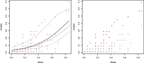
Figure 8.2. Left-hand side: fitted regression curves for the models. Breg in dotted line, VIBreg in solid line and FBreg in dashed lines. Colored dashed curves refer to the component means of the FBreg model. Right-hand side: scatterplot of stress level versus anxiety level. Red dots refer to subjects belonging to group 1
To make a comparison between competing models, a useful tool is the WAIC criterion which indicates the best model in terms of fit and the number of parameters. The FlexReg package computes the WAIC values through the waic() function. The model with the best fit to the data, understood as the lowest WAIC, is the FBreg (WAIC = −566.4), whereas the Breg (WAIC = −558.8) and VIBreg (WAIC = −558.2) models have a similar performance.
Aside from the assessment of the best model, it is of interest to evaluate any inconsistency between observed and predicted values. In a Bayesian perspective, it is convenient to compute the posterior predictive distribution, namely the distribution of unobserved values conditional on the observed data. This operation is straightforward for our flexible regression models thanks to the posterior_predict() function, the result of which is an object of class flexreg_postpred containing a matrix with the simulated posterior predictions. The plot method applied to posterior predictives returns the posterior predictive interval for each statistical unit plus the observed value of the response variable in red dots. By way of example, Figure 8.3 shows the 95% posterior predictive intervals for the VIBreg model. It is worth noting that the model provides accurate predictive intervals since all observed values are comprised within the intervals. A similar behavior also holds for the Breg and FBreg models.

Figure 8.3. 95% posterior predictive intervals for each statistical unit for the VIBreg model. The observed anxiety levels are represented with orange dots
The last inspection regarding the behavior of the regression models involves the Bayesian residuals, either raw or standardized:
where ![]() and
and ![]() are the predicted mean and variance of the response, both assessed using the posterior means of the parameters.
are the predicted mean and variance of the response, both assessed using the posterior means of the parameters.
The computation of residuals for flexible models can be done through the function called residuals(). The argument object features an object of class flexreg, which contains all the results related to the estimated model of type Breg, VIBreg or FBreg. By specifying the argument type, it is possible to compute either raw or standardized residuals. Furthermore, if the model is of FB type, the function allows us to compute also the cluster residuals that are obtained as the difference between the observed responses and the cluster means. This is achieved by simply setting cluster = T:
>residuals(object, type = c(“raw”, “standardized”), cluster = T)
It is worth noting that the cluster residuals computed for the FBreg model allow us to provide a classification of data into two clusters, as shown on the right-hand side of Figure 8.2. This result is consistent with that seen with the regression curves.
8.3.2. Reading data
The second dataset we explore, likewise from the FlexReg package, is called “Reading” and it collects data referring to a group of 44 children, 19 of whom have received a diagnosis of dyslexia. Available types of information concern the proportion of accuracy in reading tasks and the non-verbal intelligent quotient (IQ), besides the dyslexia status (DYS, being dyslexic (1) or not (0)).
This case study has been extensively analyzed within the literature on regression models for bounded responses and it is of special interest because of the presence of values at the upper boundary of the support, corresponding to children (13 out of 44) that achieved a perfect score in reading tests. One possibility is to handle this dataset by simpling transforming the response variable from (0, 1] to the open interval (0, 1). An alternative option is to analyze the dataset through an augmentation strategy.
If we assume ignorance about the dyslexic status of children, we can fit an augmented regression model where the mean and the proportion q1 are both regressed onto the IQ covariate:
Please note that q0 = 0 since there are no values at the lower limit of the support. We fit ABreg, AFBreg and AVIBreg regression models according to equation [8.6]. Each model is run 20,000 iterations with the first half as burn-in. For comparison purposes, we also fit the standard Breg, FBreg and VIBreg models by setting q1 = 0 in equation [8.6] and by simply transforming the response values from (0, 1] to the open interval (0, 1). Focusing on the models with augmentation, the AFBreg model shows excellent fit to data. Indeed, the WAIC estimated for the AFBreg model is equal to 8.1, whereas the WAIC values of the ABreg and VIBreg models are greater and equal to 12.4 and 12.6, respectively. An analogous outcome is achieved by comparing the models without augmentation: the best fit (lowest WAIC) is provided by the FBreg model (WAIC = -84.1), whereas the Breg (WAIC = -63.6) and VIBreg (WAIC = -63.2) models show a similar performance. The impact of the augmentation strategy is particularly evident from the left-hand panel of Figure 8.4. When the values at the upper boundary of the support are modeled separately from the rest of data, the effect on the regression curves for the mean of the augmented model is a shift towards the bottom with respect to the regression curve of the non-augmented model, regardless of the type of model. In both cases, with and without augmentation, the regression models of FB type generate more flat curves than the ones from competing models. This behavior is a direct consequence of the special mixture structure of the FB distribution. By way of example, if we focus on the AFBreg model (see the right-hand panel of Figure 8.4), it emerges that the model dedicates the first component to the fit of the observations with the highest scores in the reading accuracy test (without the perfect scores) which also corresponds to non-dyslexic children, whereas the second component is dedicated to the remaining part of the data cloud. Therefore, in a sense, we can conclude that the models of FB type are able to detect the clustering structure induced by the dyslexic status, which is assumed latent so far.
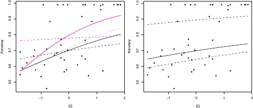
Figure 8.4. Left-hand side: fitted regression curves for the models with augmentation (violet lines) and without augmentation (black lines) refer to the Breg (dotted lines), VIBreg (solid lines) and FBreg (dashed lines) models. Right-hand side: fitted regression curve for the overall mean (solid line) and for the component means (dashed lines) of the AFBreg model
As a second step, we consider a complete model by regressing the mean, the precision, and the excess of 1s onto the quantitative covariate IQ, the dyslexic status (DYS) and their interaction. The ABreg, AFBreg and AVIBreg regression models with regression equations as in equation [8.6] have been estimated through the HMC algorithm:

The three competing models show similar fit to data, in terms of WAIC. Moreover, by looking at posterior means and credible intervals (CIs) from Table 8.1, it emerges that the dyslexic status of children plays a significant role in explaining both the probability of achieving a perfect score, the mean and the precision of the reading accuracy response variable in all competing models.
Table 8.1. Reading data: posterior means and CIs for the parameters of the AFBreg, AVIBreg and ABreg regression models together with WAIC values
| ABreg | AVIBreg | AFBreg | ||
| Parameters | Mean 95% CI | Mean 95% CI | Mean 95% CI | |
| mean | β1,0 (intercept) β1,1 (DYS) β1,2 (IQ) β1,3 (IQ×DYS) | 0.385 (0.25;0.523) 0.872 (0.347;1.341) -0.079 (-0.217;0.07) 0.438 (-0.423;1.447) | 0.389 (0.253;0.538) 0.854 (0.336;1.314) -0.078 (-0.209;0.081) 0.434 (-0.385;1.467) | 0.405 (0.236;0.585) 0.83 (0.402;1.299) -0.076 (-0.214;0.074) 0.38 (-0.39;1.305) |
| precision | β2,0 (intercept) β2,1 (DYS) β2,2 (IQ) β2,3 (IQ × DYS) | 4.434 (3.261;5.377) -2.011 (-3.471;-0.519) 0.598 (-0.549;1.651) -1.246 (-3.061;0.887) | 4.819 (3.467;6.599) -1.955 (-3.49;-0.378) 0.576 (-0.578;1.694) -1.273 (-3.21;0.883) | 4.557 (3.27;5.687) -1.557 (-3.594;0.901) 0.575 (-0.729;1.768) -1.902 (-4.885;0.885) |
| augment. | β3,0 (intercept) β3,1 (DYS) β3,2 (IQ) β3,3 (IQ × DYS) | -4.854 (-13.809;-1.575) 4.453 (0.891;13.559) 0.715 (-1.691;3.228) 0.166 (-2.378;2.708) | -4.623 (-11.454;-1.564) 4.22 (0.867;10.999) 0.719 (-1.683;3.36) 0.166 (-2.528;2.798) | -5.021 (-14.709;-1.506) 4.612 (0.9;14.286) 0.721 (-1.78;3.331) 0.153 (-2.555;2.89) |
| p k w | 0.504 (0.02;0.98) 0.566 (0.077;0.978) | 0.386 (0.009;0.987) 0.296 (0.012;0.81) | ||
| WAIC | -23.8 | -23.6 | -23.2 |
8.4. References
Aitchison, J. (1986). The Statistical Analysis of Compositional Data. Chapman and Hall, London.
Albert, J. (2009). Bayesian Computation With R, 2nd edition. Springer Science, New York.
Barrientos, A.F., Jara, A., Quintana, F.A. (2017). Fully nonparametric regression for bounded data using dependent Bernstein polynomials. Journal of the American Statistical Association, 112(518), 806–825.
Bayes, C., Bazan, J.L., de Castro, M. (2017). A quantile parametric mixed regression model for bounded response variables. Statistics and Its Interface, 10(3), 483–493.
Di Brisco, A.M., Migliorati, S., Ongaro, A. (2020). Robustness against outliers: A new variance inflated regression model for proportions. Statistical Modelling, 20(3), 274–309.
Duane, S., Kennedy, A., Pendleton, B.J., Roweth, D. (1987). Hybrid Monte Carlo. Physics Letters B, 195(2), 216–222.
Ferrari, S. and Cribari-Neto, F. (2004). Beta regression for modelling rates and proportions. Journal of Applied Statistics, 31(7), 799–815.
Frühwirth-Schnatter, S. (2006). Finite Mixture and Markov Switching Models. Springer, Berlin, Heidelberg.
Gelman, A., Carlin, J.B., Stern, H.S., Rubin, D.B. (2014). Bayesian Data Analysis, Volume 2. Taylor & Francis, Abingdon.
Lemonte, A.J. and Bazán, J.L. (2016). New class of Johnson SB distributions and its associated regression model for rates and proportions. Biometrical Journal, 58(4), 727–746.
McCullagh, P. and Nelder, J.A. (1989). Generalized Linear Models, Volume 37. CRC Press, Boca Raton, FL.
Migliorati, S., Di Brisco, A.M., Ongaro, A. (2018). A new regression model for bounded responses. Bayesian Analysis, 13(3), 845–872.
Neal, R.M. (1994). An improved acceptance procedure for the hybrid Monte Carlo algorithm. Journal of Computational Physics, 111(1), 194–203.
Qiu, Z., Song, P.X.-K., Tan, M. (2008). Simplex mixed-effects models for longitudinal proportional data. Scandinavian Journal of Statistics, 35(4), 577–596.
Smithson, M. and Verkuilen, J. (2006). A better lemon squeezer? Maximum-likelihood regression with beta-distributed dependent variables. Psychological Methods, 11(1), 54–71.
Stan Development Team (2016). Stan modeling language users guide and reference manual [Online]. Available at: https://mc-stan.org/users/documentation/.
Vehtari, A., Gelman, A., Gabry, J. (2017). Practical Bayesian model evaluation using leave-one-out cross-validation and WAIC. Statistics and Computing, 27(5), 1413–1432.
Chapter written by Agnese Maria DI BRISCO, Roberto ASCARI, Sonia MIGLIORATI and Andrea ONGARO.
- For a color version of all the figures in this chapter, see www.iste.co.uk/zafeiris/data1.zip.
- 1 https://CRAN.R-project.org/package=FlexReg.