
9
Simulation Studies for a Special Mixture Regression Model with Multivariate Responses on the Simplex
Compositional data are defined as vectors whose elements are strictly positive and subject to a unit-sum constraint. When the multivariate response is of compositional type, a proper regression model that takes account of the unit-sum constraint is required. This contribution illustrates a new multivariate regression model for compositional data that is based on a mixture of Dirichlet-distributed components. Its complex structure is offset by good theoretical properties (among which identifiability) and a greater flexibility than the standard Dirichlet regression model. We perform intensive simulation studies to evaluate the fit of the proposed regression model and its robustness in the presence of multivariate outliers. The (Bayesian) estimation procedure is performed via the efficient Hamiltonian Monte Carlo algorithm.
9.1. Introduction
Compositional data, namely proportions of some whole, are encountered in several fields of science and require proper statistical tools of analysis (Aitchison 2003). Indeed, compositional data have the peculiarity of being vector of proportions lying on the simplex space:  . The analysis of compositional data is challenging since it cannot make use of standard techniques that might lead to distorted results due to ignoring the unit-sum constraint. A fruitful strategy in the analysis of compositional data takes advantage of statistical distributions defined on the simplex. Among them, the Dirichlet distribution is a widespread distribution for a D-dimensional vector
 ![]() . A regression model based on the Dirichlet distribution is straightforward for compositional data and proves to behave satisfactorily (Campbell and Mosimann 2009; Hijazi and Jernigan 2009; Maier 2014). As a counterpart, it has some limitations among which its inability of modeling multimodality, heavy tails and the eventual presence of outliers. A convenient approach to induce multimodality and an overall increase in flexibility is to consider a mixture distribution. In this regard, we propose to resort to a special finite mixture of Dirichlet components referred to as the Extended Flexible Dirichlet (EFD) (Ongaro). Moreover, we illustrate a regression model based on the EFD distribution (Di Brisco et al. 2019). The aim of this work is to intensively study the behavior of the EFD regression model in many simulated scenarios covering some relevant statistical issues such as the presence of outliers, heavy tails and latent groups. We compare the EFD regression model with the Dirichlet one in terms of fit and estimates of the regression parameters.
. A regression model based on the Dirichlet distribution is straightforward for compositional data and proves to behave satisfactorily (Campbell and Mosimann 2009; Hijazi and Jernigan 2009; Maier 2014). As a counterpart, it has some limitations among which its inability of modeling multimodality, heavy tails and the eventual presence of outliers. A convenient approach to induce multimodality and an overall increase in flexibility is to consider a mixture distribution. In this regard, we propose to resort to a special finite mixture of Dirichlet components referred to as the Extended Flexible Dirichlet (EFD) (Ongaro). Moreover, we illustrate a regression model based on the EFD distribution (Di Brisco et al. 2019). The aim of this work is to intensively study the behavior of the EFD regression model in many simulated scenarios covering some relevant statistical issues such as the presence of outliers, heavy tails and latent groups. We compare the EFD regression model with the Dirichlet one in terms of fit and estimates of the regression parameters.
The rest of this chapter is organized as follows. Section 9.2 introduces the Dirichlet and the EFD distributions, and it shows convenient parameterizations for regression purposes. Section 9.3 outlines details on the EFD regression model. Section 9.3.1 provides an overview on the HMC algorithm, a Bayesian approach to inference especially suited for mixture models. Section 9.4 illustrates several simulation studies that have been performed to evaluate the behavior and the fit to data of the EFD regression model in comparison to the Dirichlet one.
9.2. Dirichlet and EFD distributions
A Dirichlet-distributed D-dimensional vector ![]() has a probability density function (p.d.f.) as follows:
has a probability density function (p.d.f.) as follows:
where α = (α1,... , αD)Τ, αj > 0 and ![]() . With the aim of regressing a compositional vector onto a set of covariates, it is convenient to work with an alternative parameterization based on the mean vector
. With the aim of regressing a compositional vector onto a set of covariates, it is convenient to work with an alternative parameterization based on the mean vector ![]() , where
, where ![]() for j = 1,..., D, and
for j = 1,..., D, and ![]() that represents the precision parameter of the Dirichlet distribution.
that represents the precision parameter of the Dirichlet distribution.
An EFD distributed D-dimensional vector ![]() has the following p.d.f.:
has the following p.d.f.:
where ![]() and vectors α = (α1,…, αD)Τ and τ = (τ1,…, τD)Τ have positive elements. The EFD distribution function admits the following mixture representation:
and vectors α = (α1,…, αD)Τ and τ = (τ1,…, τD)Τ have positive elements. The EFD distribution function admits the following mixture representation:
where Dir(·;·) denotes the Dirichlet distribution, and er is a vector of zeros except for the r-th element which is equal to one. It is worth noting that the EFD distribution contains the Dirichlet as an inner point when τr = 1 and ![]() for every r = 1,…, D. The p.d.f. of the EFD admits a variety of shapes including, but not limited to, uni- and multi-modal ones. Moreover, the richer parameterization of the EFD with respect to the Dirichlet allows for a more flexible modelization of the dependence structure of the composition. Finally, the EFD distribution shows several theoretical properties, i.e. some simplicial forms of dependence/independence and identifiability (Ongaro), that make it tractable from computational and inferential points of view.
for every r = 1,…, D. The p.d.f. of the EFD admits a variety of shapes including, but not limited to, uni- and multi-modal ones. Moreover, the richer parameterization of the EFD with respect to the Dirichlet allows for a more flexible modelization of the dependence structure of the composition. Finally, the EFD distribution shows several theoretical properties, i.e. some simplicial forms of dependence/independence and identifiability (Ongaro), that make it tractable from computational and inferential points of view.
To define a regression model based on the EFD, it is convenient to adopt an alternative parameterization that explicitly includes the mean vector. To this end, note that the r-th Dirichlet component in equation [9.3] has a mean vector ![]() , (where
, (where ![]() and
and ![]() , which can be interpreted as a weighted average of a common barycenter,
, which can be interpreted as a weighted average of a common barycenter, ![]() and the r-th simplex vertex er. The first-order moment of the EFD easily follows from its mixture structure:
and the r-th simplex vertex er. The first-order moment of the EFD easily follows from its mixture structure:
However, the parameterization of the EFD based on μj, pj and wj (j = 1,…, D) is not variation independent since some constraints hold between parameters, and thus the following inequalities referred to wj, j = 1,…, D, can be derived as follows:
Variation independence, whose lack is a potential issue for Bayesian inference through Monte Carlo (MC) methods, can be achieved by normalizing wj as follows:
The parameterization of the EFD distribution depending on ![]() ,
, ![]() ,
, ![]() for every j, and α+ > 0 has the double benefit of being variation independent – useful for Bayesian inference – and explicitly including the mean vector – useful for regression purposes.
for every j, and α+ > 0 has the double benefit of being variation independent – useful for Bayesian inference – and explicitly including the mean vector – useful for regression purposes.
9.3. Dirichlet and EFD regression models
Since both parameterizations of the Dirichlet and of the EFD illustrated in section 9.2 explicitly include the mean vector μ, it is possible to derive a regression model for compositional data. Let Y = (Y1,…, Yn)Τ be the response matrix such that Yi, for i = 1,…, n, is a D-dimensional vector on the simplex, and let X = (x1,…, xn)Τ be the design matrix such that xi are (K + 1)-dimensional vectors. The mean vector νi of Yi can be regressed onto a set of covariates in accordance with a GLM strategy (McCullagh and Nelder 1989). Indeed, since νi lies on the simplex, a multinomial logit link function can be adopted as follows:
where ![]() is the vector of covariates, and βj = (βj0,βj1, …, βjK)Τ is a vector of regression coefficients. Please note that the Dth category is conventionally fixed as baseline, so that βDk = 0 for k = 0, 1,…, K, and thus:
is the vector of covariates, and βj = (βj0,βj1, …, βjK)Τ is a vector of regression coefficients. Please note that the Dth category is conventionally fixed as baseline, so that βDk = 0 for k = 0, 1,…, K, and thus:

If Yi are Dirichlet distributed, we recover the Dirichlet regression (DirReg) model (Hijazi and Jernigan 2009; Maier 2014) by substituting νij with ![]() in equation [9.6]. Similarly, if Yi are EFD distributed, we get the EFD regression (EFDReg) model (Di Brisco et al. 2019) by replacing νij with μij in equation [9.6].
in equation [9.6]. Similarly, if Yi are EFD distributed, we get the EFD regression (EFDReg) model (Di Brisco et al. 2019) by replacing νij with μij in equation [9.6].
9.3.1. Inference and fit
To obtain estimates of the unknown parameters of EFDReg and DirReg models, we favor a Bayesian approach. This choice is mainly motivated by the difficulty, both computational and analytical, of likelihood-based inferential approaches in dealing with complex models such as mixtures. Conversely, the finite mixture structure of the EFD distribution can be advantageously treated as an incomplete data problem in a Bayesian paradigm (Frühwirth-Schnatter 2006). Among the MC methods, a recent solution is the Hamiltonian Monte Carlo (HMC) (Neal 1994) algorithm, a generalization of the Metropolis algorithm which combines Markov Chain Monte Carlo (MCMC) and deterministic simulation methods. The (simulated) posterior distributions of the unknown parameters are simulated on the basis of the full likelihood and prior distributions. With regard to choice of priors, we adopt non- or weakly informative priors to induce the minimum impact on the posteriors (Albert 1987), and suppose prior independence. We select a multivariate normal with zero mean vector and diagonal covariance matrix with “large” values of the variances as non-informative prior for the regression parameters βj . Moreover, we adopt a Uniform(0, 1) prior for ![]() , and a Dirichlet prior with hyperparameter 1 for the vector p. Finally, we use a Gamma(g, g) prior, with g “small” and equal to 0.001, for the precision parameter α+. Among the variety of fitting criteria, we favor the Watanabe-Akaike information criterion (WAIC) (Vehtari et al. 2017) because it is fully Bayesian and well-defined for non-regular models such as mixture ones as well. As a general rule, the smaller the criterion is, the better the model fit.
, and a Dirichlet prior with hyperparameter 1 for the vector p. Finally, we use a Gamma(g, g) prior, with g “small” and equal to 0.001, for the precision parameter α+. Among the variety of fitting criteria, we favor the Watanabe-Akaike information criterion (WAIC) (Vehtari et al. 2017) because it is fully Bayesian and well-defined for non-regular models such as mixture ones as well. As a general rule, the smaller the criterion is, the better the model fit.
9.4. Simulation studies
To compare the performances of the EFDReg and DirReg models, we simulated a variety of scenarios that cover many potentially tricky problems among which multimodality, as well as the presence of heavy tails, outliers and latent groups. In the following, we illustrate the samples’ simulation schemes and the main inferential results for each scenario. We took advantage of the HMC algorithm for estimating the vector of unknown parameters ![]() . The algorithm is easily implemented by the Stan modeling language (Stan Development Team 2016). We ran chains of length 10,000 and we discarded the first half. Moreover, we checked the convergence to the target distribution through graphical tools, such as trace-plots, density-plots and autocorrelation-plots, as well as diagnostic measures such as the potential scale reduction factor, the effective sample size and the Raftery–Lewis test (Gelman et al. 2013). Each scenario is replicated 500 times to evaluate MC estimates. Computational times are of approximately 60 seconds for DirReg and 300 seconds for EFDReg.
. The algorithm is easily implemented by the Stan modeling language (Stan Development Team 2016). We ran chains of length 10,000 and we discarded the first half. Moreover, we checked the convergence to the target distribution through graphical tools, such as trace-plots, density-plots and autocorrelation-plots, as well as diagnostic measures such as the potential scale reduction factor, the effective sample size and the Raftery–Lewis test (Gelman et al. 2013). Each scenario is replicated 500 times to evaluate MC estimates. Computational times are of approximately 60 seconds for DirReg and 300 seconds for EFDReg.
Fitting study: First, we evaluated some fitting studies by simulating from Dirichlet (scenario (i)) and EFD (scenario (ii)) regression models. The objective of these studies is to analyze the goodness of fit and estimates of regression coefficients. The sample size is n = 150, and the multivariate response lies on the three-part simplex. In both scenarios, a quantitative covariate x, uniformly distributed in (−0.5, 0.5), is included in the regression model for the mean (see equation [9.6]), with regression coefficients set equal to β10 = 1, β11 = 2, β20 = 0.5, β21 = −3. In scenario (i), the response is Dirichlet distributed and the precision parameter is α+ = 50. In scenario (ii), the response is EFD distributed, and the remaining parameters are fixed equal to α+ = 50, p = (1/3, 1/3, 1/3)Τ and ![]() . Ternary plots and scatterplots of each element of the composition yij, j = 1, 2, 3, versus the quantitative covariate x are shown in Figures 9.1 (scenario (i)) and 9.2 (scenario (ii)). It is worth noting the absence of whatever cluster in scenario (i), while in scenario (ii) it is clear the presence of clusters and multiple modes.
. Ternary plots and scatterplots of each element of the composition yij, j = 1, 2, 3, versus the quantitative covariate x are shown in Figures 9.1 (scenario (i)) and 9.2 (scenario (ii)). It is worth noting the absence of whatever cluster in scenario (i), while in scenario (ii) it is clear the presence of clusters and multiple modes.
Presence of outliers: To evaluate the behavior of the DirReg and EFDReg models in the presence of outliers, we perturbed scenario (i) according to the following perturbation scheme. We randomly selected 15 observations (10% of the sample size) and we applied the perturbation operation defined as ![]() , , where y and δ are the vectors on the simplex playing the roles of perturbed and perturbing element, respectively. Moreover, the closure operation
, , where y and δ are the vectors on the simplex playing the roles of perturbed and perturbing element, respectively. Moreover, the closure operation ![]() is defined as
is defined as ![]() with
with ![]() and qj > 0, ∀ j = 1,…, D. The neutral element of the perturbation operation is δ = (1/D,…, 1/D)Τ, so that if element yj is perturbed by δj greater (lower) than 1/D, the perturbation is upward (downward). We set three scenarios of perturbation by fixing the perturbing element δ equal to (0.86, 0.07, 0.07)Τ in scenario (I), (0.07, 0.86, 0.07)Τ in scenario (II) and (0.07, 0.07, 0.86)Τ in scenario (III).
and qj > 0, ∀ j = 1,…, D. The neutral element of the perturbation operation is δ = (1/D,…, 1/D)Τ, so that if element yj is perturbed by δj greater (lower) than 1/D, the perturbation is upward (downward). We set three scenarios of perturbation by fixing the perturbing element δ equal to (0.86, 0.07, 0.07)Τ in scenario (I), (0.07, 0.86, 0.07)Τ in scenario (II) and (0.07, 0.07, 0.86)Τ in scenario (III).

Figure 9.1. Representations of one replication from scenario (i)
Figures 9.3, 9.4 and 9.5 show the effect of perturbation on the Dirichlet-distributed responses. In all plots, the perturbed points are in light-blue while unperturbed points are in black. Looking at the scatterplots, we can observe that scenario (I) assumes some outlying observations upward for the first element and downward for the second and third elements of the composition; this is coherent with the chosen vector δ that has the first element greater than 0.5 and the second and third elements lower than 0.5. Instead, in scenarios (II) and (III), the second and third elements of the composition respectively are perturbed upward while the remaining elements are perturbed downward. Focusing on the ternary plots, it is worth noting that the effect of perturbation in scenario (III) is clearly visible in that the group of perturbed values, in blue, is well-separated from the remaining points, in black. The overall effect of perturbing vector δ = (0.07, 0.07, 0.86)Τ is thus to shift the cloud of points towards the bottom-right vertex of the plot. Conversely, in scenarios (I) and (II), the perturbed points are overall shifted towards the bottom-left and top vertex of the ternary plot, respectively, i.e. in a region with a higher presence of unperturbed points.
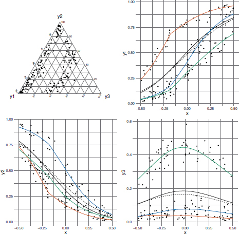
Figure 9.2. Representations of one replication from scenario (ii)
Presence of latent groups: The following simulation study explores the case of the presence of a latent (unobserved) covariate that induces the occurrence of clusters. Therefore, data are simulated by including an additional covariate in the regression model that is assumed unknown, not accounted for by the estimates of the Dirichlet and EFDReg models. In particular, we replicated the generating mechanism of fitting study (i) by adding a latent dichotomous covariate (scenario (a)) and a latent covariate with three categories (scenario (b)). In scenario (a), the additional regression coefficients are β12 = −1 and β22 = 2, and in scenario (b), they also include β13 = 0.5 and β23 = −3. With respect to the dichotomous covariate of scenario (a), the categories have probabilities of 0.3 and 0.7. In scenario (b), the three categories of the latent covariate have probabilities of 0.3, 0.15, and 0.55. Figures 9.6 and 9.7 show one random replication from scenarios (a) and (b) with latent groups, respectively. In the ternary plots, points are colored and shaped according to their belonging to the latent groups. The existence of two and three clusters respectively is particularly visible from the scatterplots referred to the first and second elements of the composition.
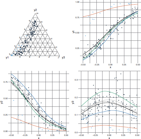
Figure 9.3. Scenario (I). Perturbed points are in light-blue and unperturbed points are in black

Figure 9.4. Scenario (II). Perturbed points are in light-blue and unperturbed points are in black
Generic mixture of Dirichlet: Finally, we evaluate the case of a generic mixture of two Dirichlet distributions: ![]() . Please note that the mixture structure is not of EFD type. Both Dirichlet distributions have the same regression model equal to that of scenario (i), but they differ in their precision parameters that are equal to
. Please note that the mixture structure is not of EFD type. Both Dirichlet distributions have the same regression model equal to that of scenario (i), but they differ in their precision parameters that are equal to ![]() and
and ![]() , respectively. The mixing proportion parameter π is equal to 0.3.
, respectively. The mixing proportion parameter π is equal to 0.3.
The generic mixture of two Dirichlet distributions has been chosen to induce heavier tails than that of the Dirichlet. The ternary plot on the top left panel of Figure 9.8 shows one random replication from the generic mixture where the green points belong to the first component of the mixture and the orange triangles belong to the second component. We can observe that the majority of points (belonging to the second component of the mixture) are placed on the ternary plot and on the scatterplots similarly to scenario (i). At the same time, the group of data coming from the Dirichlet with the smaller precision parameter is far from the remaining points. Focusing on the scatterplots referred to the first and second elements of the composition (top right and bottom left panels of Figure 9.8), it is worth noting that the responses belonging to the first component of the mixture, that is, the one with the smaller precision parameter, depart from the data cloud both upward and downward.

Figure 9.5. Scenario (III). Perturbed points are in light-blue and unperturbed points are in black
9.4.1. Comments
Table 9.1 shows the WAIC values in all simulation studies. In fitting study (i), where the data generating mechanism is Dirichlet, the WAIC of both models is comparable, while in all remaining scenarios the EFDReg model is far better than the DirReg one. The superiority in fit of the EFDReg model is particularly noticeable in fitting study (ii), in all scenarios with outliers, and in the presence of a latent group induced by a dichotomous covariate (scenario (a)). Scenario (b) (i.e. three latent groups) and the scenario from a generic mixture of two Dirichlet distributions are particularly challenging and result in a difficulty in fit for both models. Nevertheless, the EFDReg model is capable of providing a better adaptation to data (lower WAIC) than the DirReg.

Figure 9.6. Representations of one replication in the presence of latent groups, scenario (a)
Let us now analyze and comment on the posterior means and MSEs for the Dirichlet and EFD regression models in all scenarios. All results can be found in Tables 9.2, 9.3 and 9.4. Moreover, we deepen the analysis of the two models by inspecting the regression curves that are superimposed on the scatterplots in Figures 9.1–9.8. In all figures, black solid lines refer to the EFD model and black dashed lines refer to the Dirichlet one. In some scenarios only the solid line appears meaning that the regression curves of both models are almost coincident. Colored lines are referred to the component means λ1 (orange), λ2 (blue), and λ3 (green) of the EFDReg model.
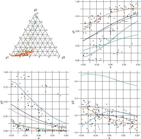
Figure 9.7. Representations of one replication in the presence of latent groups, scenario (b)
Results about the fitting study with Dirichlet-distributed data (scenario (i)), can be found in the second and third columns of Table 9.2. It is worth noting that both models provide precise estimates for the regression parameters and similar MSEs. This is confirmed by almost identical regression curves for the Dirichlet (black dashed line) and EFD (black solid line) models (see scatterplots in Figure 9.1). The DirReg model also provides a precise estimate for the precision parameter α+, while the EFDReg model slightly overestimates it. Looking at the additional parameters of the EFDReg model, we can observe that the adaptation to Dirichlet-distributed data is achieved thanks to equally weighted (estimated pj equal to approximately 0.3 for j = 1, 2, 3) and close component means (small estimated distances ![]() between components). Graphically, the regression curves referred to component means of the EFDReg model (colored solid lines) are close together and with similar distances.
between components). Graphically, the regression curves referred to component means of the EFDReg model (colored solid lines) are close together and with similar distances.

Figure 9.8. Representations of one replication of a generic mixture of two Dirichlet distributions
Table 9.1. WAIC values in the simulation studies
| Scenario | Fitting studies | Presence of outliers | Latent groups | Generic mixture | ||||
| (i) | (ii) | (I) | (II) | (III) | (a) | (b) | ||
| Dir | -948.029 | -512.614 | -633.131 | -623.990 | -565.643 | -430.142 | -611.100 | -557.735 |
| EFD | -946.140 | -883.605 | -849.742 | -814.106 | -833.923 | -770.366 | -764.415 | -593.995 |
In fitting study (ii), the EFDReg model adapts well to data and provides precise estimates with low MSEs and SEs for all the parameters (see Table 9.4). On the contrary, the DirReg model, in trying to adapt to data, estimates a considerably lower precision than the true one, and it also fails to correctly estimate some of the regression parameters. From scatterplots in Figure 9.2 it emerges that the regression curves for the EFDReg model adapt very well to data (both for the overall mean and for the component means), while they are systematically more flat for the DirReg model.
Table 9.2. Posterior means for the Dirichlet and EFD regression models in fitting study (i) and in scenarios (a) and (b) with latent groups. MSEs for the regression coefficients and SEs for remaining parameters are in parenthesis
| Scenario | Fitting study (i) | Latent groups (a) | Latent groups (b) | |||
| Model | Dir | EFD | Dir | EFD | Dir | EFD |
| β10 = 1 | 1.001 (0.001) | 1.001 (0.001) | 0.514 (0.231) | 0.850 (0.024) | 0.756 (0.060) | 1.104 (0.012) |
| β11 = 2 | 1.998 (0.018) | 1.992 (0.018) | 1.567 (0.203) | 1.665 (0.131) | 1.328 (0.461) | 1.299 (0.510) |
| β20 = 0.5 | 0.501 (0.001) | 0.502 (0.001) | 0.883 (0.148) | 1.275 (0.605) | -0.600 (1.213) | -0.044 (0.230) |
| β21 = –3 | -3.006 (0.021) | -2.998 (0.021) | -1.963 (1.086) | -2.096 (0.835) | -1.568 (2.096) | -1.634 (1.945) |
| α+ = 50 | 50.052 (4.338) | 53.636 (5.473) | 5.894 (0.258) | 21.241 (2.023) | 3.033 (0.121) | 5.389 (0.600) |
| p1 | — | 0.290 (0.111) | — | 0.640 (0.030) | — | 0.582 (0.071) |
| p2 | — | 0.315 (0.119) | — | 0.353 (0.030) | — | 0.409 (0.071) |
| p3 | — | 0.395 (0.116) | — | 0.007 (0.002) | — | 0.009 (0.001) |
| — | 0.149 (0.031) | — | 0.608 (0.032) | — | 0.584 (0.037) | |
| — | 0.146 (0.041) | — | 0.707 (0.021) | — | 0.780 (0.019) | |
| — | 0.151 (0.032) | — | 0.461 (0.056) | — | 0.421 (0.012) | |
The estimates of the unknown parameters in the three scenarios with outliers are shown in Table 9.3. Moreover, the regression curves of the Dirichlet and EFD models are plotted on the scatterplots in Figures 9.3, 9.4 and 9.5 referred to scenarios (I), (II), and (III), respectively. The estimates of the regression parameters of the Dirichlet and EFD models are affected by the presence of outliers. The element of flexibility used by the DirReg model in order to adapt to data that depart from the Dirichlet distribution is given by the precision parameter, that is systematically underestimated in all scenarios with outliers. Conversely, the EFDReg model can take advantage of its special mixture structure to better adapt to data. It is worth noting that in all scenarios with outliers, one component of the mixture is dedicated to the group of perturbed values as indicated by the corresponding pj estimate which is around 0.1. The remaining two components equally describe the remaining majority of unperturbed data with estimates of pj’s between 0.3 and 0.5. The analysis of the regression curves allows us to better understand the different behavior of the DirReg and EFDReg models. The regression curves of the DirReg model are slightly shifted with respect to the regression curves of the DirReg in the scenario without perturbation (dotted lines in Figures 9.3–9.5) in the direction of the perturbed values. Instead, looking at the component means of the EFD we note that the first, second and third components of the mixture are entirely dedicated to model the subgroup of outliers in scenarios (I), (II) and (III).
Table 9.3. Posterior means for the Dirichlet and EFD regression models in scenarios (I), (II) and (III) with outliers. MSEs for the regression coefficients and SEs for remaining parameters are in parenthesis
| Scenario | Outliers (I) | Outliers (II) | Outliers (III) | |||
| Model | Dir | EFD | Dir | EFD | Dir | EFD |
| β10 = 1 | 1.134 (0.019) | 1.183 (0.036) | 0.914 (0.008) | 0.992 (0.001) | 0.699 (0.092) | 0.682 (0.103) |
| β11 = 2 | 1.840 (0.065) | 1.748 (0.081) | 1.871 (0.030) | 1.924 (0.022) | 1.830 (0.075) | 1.962 (0.014) |
| β20 = 0.5 | 0.472 (0.002) | 0.502 (0.002) | 0.683 (0.035) | 0.898 (0.180) | 0.262 (0.058) | 0.192 (0.097) |
| β21 = –3 | -2.693 (0.112) | -2.895 (0.035) | -2.728 (0.123) | -2.349 (0.462) | -2.658 (0.165) | -2.929 (0.020) |
| α+ = 50 | 14.930 (1.177) | 37.754 (7.304) | 15.012 (1.205) | 35.590 (4.526) | 13.328 (0.940) | 41.561 (4.424) |
| p1 | — | 0.121 (0.170) | — | 0.553 (0.282) | — | 0.479 (0.228) |
| p2 | — | 0.372 (0.300) | — | 0.147 (0.086) | — | 0.434 (0.229) |
| p3 | — | 0.507 (0.309) | — | 0.300 (0.281) | — | 0.087 (0.008) |
| — | 0.744 (0.054) | — | 0.281 (0.084) | — | 0.155 (0.050) | |
| — | 0.265 (0.090) | — | 0.706 (0.057) | — | 0.153 (0.052) | |
| — | 0.272 (0.101) | — | 0.265 (0.101) | — | 0.613 (0.030) | |
Results concerning the presence of some latent groups in data are shown in the last four columns of Table 9.2. The estimates of regression parameters are biased for both models. Once again, the DirReg model tries to adapt to data by estimating a very low value for the precision parameter, nevertheless this results in a very poor fit. The regression curves of the DirReg model, reported in Figures 9.6 and 9.7, severely miss the data cloud, particularly in scenario (a). The EFDReg model has a satisfactory behavior in scenario (a) where the latent covariate has two categories with probabilities of 0.3 and 0.7. These latent clusters are grasped by the EFDReg model with an estimate equal to 0.64 and 0.353 for the mixing proportions p1 and p2 of the first and second component, and an estimate close to zero for p3. This is clearly reflected by the regression curves of the component means of the EFD model plotted in Figures 9.6 and 9.7. It is worth noting that the orange and blue lines λ1 and λ2 perfectly fit the two data clouds. On the contrary, the green line λ3 has a very poor fit, but this does not affect the overall fit of the model since the third component of the mixture has a probability of occurrence around zero. Scenario (b) is more challenging for the EFDReg model. Please recall that this scenario assumes the existence of a latent covariate having three categories with probabilities of 0.3, 0.15 and 0.55. Nevertheless, the EFD model is able to capture only two out of the three latent clusters, as witnessed by the estimate of the third mixing proportion p3 which is close to zero. A look at the regression curves of the component means of the EFD model (Figure 9.7) better explains this behavior. The first scatterplot, referred to the first element of the response, shows a good fit of the orange curve λ1. The remaining two curves λ2 and λ3 are unable to describe the two visible clusters of data since they are placed in the middle. In the second scatterplot, referred to second elements of the response, the blue curve adapts well to one cluster, the green and orange ones are almost overlapping and fit a second cluster well while a third cluster of data is missed by all curves. In the third scatterplot, referred to the third element of the response, the blue and orange curves cross the data cloud, but the green one misses it completely. Overall, the EFDReg model has an excessively rigid mixture structure to adapt to this scenario well, whilst remaining a far better model than the Dirichlet one.
Table 9.4. Posterior means for the Dirichlet and EFD regression models in fitting study (ii) and in case of a generic mixture of Dirichlet. MSEs for the regression coefficients and SEs for remaining parameters are in parenthesis
| Scenario | Fitting study (ii) | Scenario | Generic mixture | ||
| Model | Dir | EFD | Model | Dir | EFD |
| β10 = 1 | 1.087 (0.015) | 1.014 (0.010) | β10 = 1 | 1.006 (0.010) | 0.947 (0.010) |
| β11 = 2 | 1.990 (0.069) | 1.999 (0.012) | β11 = 2 | 2.063 (0.149) | 1.967 (0.083) |
| β20 = 0.5 | 0.752 (0.068) | 0.511 (0.010) | β20 = 0.5 | 0.501 (0.014) | 0.457 (0.014) |
| β21 = –3 | -2.409 (0.395) | -3.009 (0.014) | β21 = –3 | -2.967 (0.189) | -2.866 (0.159) |
| β+ = 50 | 6.444 (0.306) | 50.153 (4.253) | β+ | 5.619 (0.892) | 6.877 (1.684) |
| p1 = 1/3 | — | 0.335 (0.024) | p1 | — | 0.149 (0.239) |
| p2 = 1/3 | — | 0.335 (0.034) | p2 | — | 0.189 (0.293) |
| p3 = 1/3 | — | 0.331 (0.035) | p3 | — | 0.662 (0.353) |
| — | 0.601 (0.016) | — | 0.563 (0.230) | ||
| — | 0.199 (0.032) | — | 0.553 (0.229) | ||
| — | 0.694 (0.029) | — | 0.732 (0.153) | ||
The last two columns of Table 9.4 show the estimates in case observations come from a generic mixture of two Dirichlet distributions. It is worth recalling that this scenario assumes that the second mixture component follows the same Dirichlet distribution as in scenario (i), and the first component differs from the second one because of the presence of a lower precision parameter. Both the DirReg and EFDReg models provide reasonably unbiased estimates of the regression parameters, despite the MSEs being greater than the ones in scenario (i). To confirm this, the regression curves (dashed and solid lines in Figure 9.8) adapt well to the majority of observations and are almost overlapping. The presence of a group of data, around 30%, coming from the Dirichlet distribution with a lower precision parameter forces the DirReg model to provide a low estimate of the precision parameter in trying to adapt to data. The EFDReg performs better than the DirReg model since it is capable of recognizing the presence of some clusters in data. In particular, it dedicates the third component to describing the majority of data, indeed the estimate of p3 is approximately equal to 0.7. Instead, the first and second components are dedicated to data coming from the second component of the generic mixture, and they show similar estimates of all parameters (pj and ![]() ). In this regard, the green curve is near the solid one, particularly in the scatterplots referred to the first and second elements of the composition. Differently, the blue and orange curves fit the values from the second component of the generic mixture, and they are placed either upward or downward with respect to the majority of points in the scatterplots.
). In this regard, the green curve is near the solid one, particularly in the scatterplots referred to the first and second elements of the composition. Differently, the blue and orange curves fit the values from the second component of the generic mixture, and they are placed either upward or downward with respect to the majority of points in the scatterplots.
9.5. References
Aitchison, J. (2003). The Statistical Analysis of Compositional Data. The Blackburn Press, London.
Albert, J. (1987). Bayesian computation with R. ASA Proceedings of Section on Statistical Graphics.
Campbell, G. and Mosimann, J.E. (2009). Multivariate analysis of size and shape: Modelling with the Dirichlet distribution. ASA Proceedings of Section on Statistical Graphics, 93–101.
Di Brisco, A.M., Ascari, R., Migliorati, S., Ongaro, A. (2019). A new regression model for bounded multivariate responses. Smart Statistics for Smart Applications – Book of Short Papers SIS, 817–822.
Frühwirth-Schnatter, S. (2006). Finite Mixture and Markov Switching Models. Springer Science + Business Media, New York.
Gelman, A., Carlin, J.B., Stern, H.S., Dunson, D.B., Vehtari, A., Rubin, D.B. (2013). Bayesian Data Analysis, 3rd edition. CRC Press, London.
Hijazi, R.H. and Jernigan, R.W. (2009). Modelling compositional data using Dirichlet regression models. Journal of Applied Probability and Statistics, 4, 77–91.
Maier, M.J. (2014). Dirichletreg: Dirichlet regression for compositional data in R. Paper, Research Report Series, University of Economics and Business, Vienna.
McCullagh, P. and Nelder, J. (1989). Generalized Linear Models. Chapman & Hall, London.
Neal, R.M. (1994). An improved acceptance procedure for the hybrid Monte Carlo algorithm. Journal of Computational Physics, 111(1), 194–203.
Ongaro, A., Migliorati, S., Ascari, R., Ongaro et al. (2020). A new mixture model on the simplex. Statistics and Computing [Online]. Available at: https://doi.org/10.1007/s11222-019-09920-x.
Stan Development Team (2016). Stan modeling language users guide and reference manual [Online]. Available at: http://mc-stan.org/.
Vehtari, A., Gelman, A., Gabry, J. (2017). Practical Bayesian model evaluation using leave-one-out cross-validation and WAIC. Statistics and Computing, 27(5), 1413–1432.
Chapter written by Agnese Maria DI BRISCO, Roberto ASCARI, Sonia MIGLIORATI and Andrea ONGARO.
For a color version of all the figures in this chapter, see www.iste.co.uk/zafeiris/data1.zip.