
10
Numerical Studies of Implied Volatility Expansions Under the Gatheral Model
The Gatheral model is a three-factor model with mean-reverting stochastic volatility that reverts to a stochastic long-run mean. This chapter reviews previous analytical results on the first- and second-order implied volatility expansions under this model. Using the Monte Carlo simulation as the benchmark method, numerical studies are conducted to investigate the accuracy and properties of these analytical expansions. Moreover, a partial calibration procedure is proposed using these expansions. This calibration procedure is implemented on real market data of daily implied volatility surfaces for an underlying market index and an underlying equity stock for periods both before and during the Covid-19 crisis.
10.1. Introduction
The classical Black–Scholes option pricing model assumes that the underlying asset follows a geometric Brownian motion with constant volatility, but there are a significant number of model extensions to ease this assumption of constant volatility. One of the recent and popular extensions is the Gatheral model, given in Gatheral (2008), where a double-mean-reverting market model is considered. The same model is later considered in Bayer et al. (2013).
Our object of interest is the asymptotic expansions of implied volatility under the Gatheral model presented in earlier research in Albuhayri et al. (2021). Albuhayri et al. (2021) obtained such asymptotic expansions by applying the Taylor formula of the implied volatility given in Pagliarani et al. (2017) to the Gatheral model. Applying this general Taylor formula to a specific three-factor model is a non-trivial task.
In Albuhayri et al. (2021), only analytical formulas were obtained. Therefore, there is a need for a thorough numerical study on the performances of these asymptotic expansions as approximation formulas for the implied volatility. Moreover, it is of practical interest to investigate how these approximation formulas can be used for calibrating the model to real data. This chapter addresses these two issues for the first- and second-order implied volatility expansions. The contribution of this chapter is to:
- 1) clarify for which range of option parameters the first- and second-order expansions give reasonable approximations;
- 2) propose a convenient and straightforward partial calibration procedure and implement it to synthetic and real market data.
Since there is no exact analytical formula on the implied volatility under the Gatheral model, we use the Monte Carlo simulation to generate benchmark (reference) values of implied volatilities for the numerical study on the performances of the asymptotic expansions.
Calibration means finding model parameters such that the model is consistent with the market data. In terms of option pricing models, we often minimize an error function on the differences between the market and model implied volatilities. In contrast to the time-consuming Monte Carlo simulation method, an analytical formula of the implied volatility model is beneficial for calibration purposes. For a general overview of model calibration to option data, we refer to Hilpisch (2019).
For the calibration task, we take advantage of the simple polynomial form of the implied volatility approximation formulas associated with the first- and second-order asymptotic expansion in order to propose a simple partial calibration procedure. By saying partial calibration, we mean that only a part of the original model parameters or a grouped form of them can be calibrated. However, such partial calibration is still useful as an intermediate step towards the final local optimization problem on the full calibration, which is a standard procedure. Moreover, our partial calibration reveals easily applicable values, like the present volatility level. It should be mentioned that Fouque et al. (2011) have proposed a calibration procedure under a different three-factor model using a polynomial form of the implied volatility. The asymptotic expansion in their work was obtained under the assumption of a fast mean-reverting volatility component together with a slow mean-reverting volatility component.
This chapter proceeds as follows. The first- and second-order asymptotic expansions of implied volatility under the Gatheral model are reviewed in section 10.2. The numerical studies on the performances of approximations associated with these expansions are presented in section 10.3. In section 10.4, a partial calibration procedure is proposed and synthetic and real data calibration is conducted. Finally, section 10.5 gives the conclusion and future work.
10.2. Asymptotic expansions of implied volatility
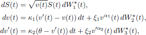
In practice, market prices of options cannot be explained by the Black–Scholes model. One possible solution to this problem is as follows. Following Dupire (1997), we postulate that under a martingale measure the underlying asset price S(t), t ∈ [0, T] satisfies the following equation:
where s is a deterministic positive number and the coefficient η(t, S(t)) is called the local volatility function.
A more recent and general extension is given in Pagliarani et al. (2017). Assuming that under a martingale probability measure, the market model is described by a ℝd-valued stochastic process (S(t), Y2(t),…, Yd(t))⊤ that satisfies the following system of stochastic differential equations:
where 2 ≤ i ≤ d and Y(t) is a vector with components Yi(t), y ∈ ℝd−1 is a deterministic vector, and the time t correlation matrix of the ℝd-valued stochastic process with components ![]() ) has entries:
) has entries:
In the rest of this chapter, we refer to this model as a local stochastic volatility model.
The model under consideration is the Gatheral model from this family of local stochastic volatility models. The Gatheral model is a double-mean-reverting market model proposed by Gatheral (2008). In a subsequent publication, Bayer et al. (2013), the model is given as follows:
and the time t correlation matrix of the ℝ3-valued stochastic process with components ![]() has entries:
has entries:
The reason why we choose this model was described by Bayer et al. (2013) as follows:
Thus variance mean-reverts to a level that itself moves slowly over time with the state of the economy.
By setting α1 = α2 = 0.5 in the Gatheral model above, we have what is known as the Double Heston model. Similarly, setting α1 = α2 = 1 leads to the Double Lognormal model.
The European call options are traded on the market; however, the stock’s volatility, σ, is not directly observable. A possible solution to this problem follows. It is well known that the Black–Scholes price with zero interest rate satisfies the following boundary value problem for the Black–Scholes partial differential equation:
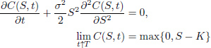
with (S, t) ∈ (0, ∞) × (0,T). Berestycki et al. (2002) describe a possible solution as follows:
[…] it is common practice to start from the observed prices and invert the closed-form solution to (2) in order to find that constant σ – called implied volatility – for which the solution to (2) agrees with the market price at today’s value of the stock.
Note that their equation (2) is our equation [10.2].
As addressed in the introduction, an analytical formula of the implied volatility under the Gatheral model is useful for the model calibration purpose in particular. Such a formula can also be used for European option valuation by plugging in the model implied volatility into the famous Black–Scholes option pricing formula.
In Albuhayri et al. (2021), we proved the following results under the model (equation [10.1]).
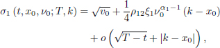
THEOREM 10.1.– The asymptotic expansion of order 1 of the implied volatility has the form:
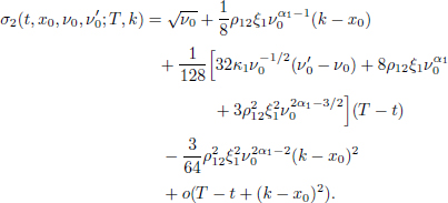
THEOREM 10.2.– The asymptotic expansion of order 2 of the implied volatility has the form:
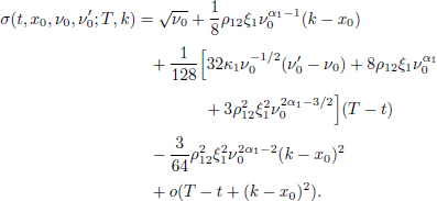
Here, x0 = ln S0, k is the logarithmic strike price of a European call option, the quantity k − x0 will be called the log-moneyness in the rest of this chapter. Discarding the o(·) terms, we can use these expansions as approximation formulas for the model implied volatility.
10.3. Performance of the asymptotic expansions
In this section, we conduct numerical studies on the performance of these asymptotic expansions of the implied volatility. We focus on two special cases of the Gatheral model given in equation [10.1]: the Double Heston model and the Double Lognormal model. As there is no exact formula for the implied volatility under the Gatheral model, we employ the Monte Carlo simulation to generate benchmark values for the implied volatilities. All errors are calculated by treating the benchmark values from the Monte Carlo simulation as the exact values.
The parameters used for the simulation are given in Table 10.1. Here, the initial asset price is denoted by S0, the number of steps by M, the number of paths by I, and the rest are the Gatheral model parameters.
Table 10.1. Fixed parameters used for the numerical study
| Parameter | Value | Parameter | Value | Parameter | Value |
| r | 0 | κ1 | 5.5 | ρ12 | −0.4 |
| S0 | 100 | κ2 | 0.1 | ρ13 | 0 |
| M | 150 | υ0 | 0.05 | ρ23 | 0 |
| I | 10000000 | 0.04 | θ | 0.078 |
The number of steps, M, is larger for longer maturities. The parameter choices come from Bayer et al. (2013). Here, ρ13 = ρ23 = 0 is the most realistic situation.
Indeed, the correlation between the underlying asset and the long-run mean and the correlation between the volatility and its long-run mean should be close to zero. Correlation ρ12 is set to be negative as the underlying price and the volatility are usually negatively correlated.
For the benchmark Monte Carlo simulation, the Euler–Maruyama discretization scheme in combination with the moment matching method for the set of generated standard normal pseudo-random numbers, volatility and underlying asset’s price series was used (see, for example, Hilpisch (2019) for the moment-matching method). In addition, the value of a forward contract on the same underlying, and with the same strike and maturity was used as a control variate. This is because the exact value of the forward contract can be easily computed.
By setting α1 = α2 = 0.5 in the Gatheral model, the Double Heston model is obtained. Similarly, α1 = α2 =1 leads to the Double Lognormal model.
We consider 130 options with 10 maturities (30, 60, 91, 122, 152, 182, 273, 365, 547 and 730 calendar days) and with log-moneyness between −0.2 and 0.2 and report the proportion of options that can be approximated within a relative error of 5% using the second-order asymptotic expansion below.
For the Double Heston model, this proportion is 45% of all options. However, the accuracy becomes much higher for options with log-moneyness between −0.1 and 0.07, and maturities from 30 days to 1 year.
Figures 10.1 and 10.2 are the examples of the asymptotic expansions of orders 1 and 2 of the implied volatility, and the benchmark values for two different times to maturities, 30 days and 1 year, respectively. The number of time steps was M = 300. From this example, it may be seen that the asymptotic expansion of order 2 gives better approximations, as expected. In addition, note that Figure 10.2 represents the worst case for maturities ranging from 30 days to 1 year. The second-order approximations are more accurate for maturities shorter than 1 year.
Similarly, for the Double Lognormal model, with the second-order expansion, the corresponding proportion of options that can be approximated within a relative error of 5% is around 55%. For options with log-moneyness between −0.07 and 0.096, and maturities from 30 days to 1 year options, the accuracy again becomes higher.
For the first-order expansion, the approximation is decent with relative error less than 5% only for options with a maturity as short as 30 days, and log-moneyness between −0.1 and 0.07.
Similar experiments have been done for other values of α1, α2, for example, α1 = α2 = 0.94, the results are alike.
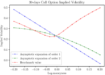
Figure 10.1. An example of the asymptotic expansions of orders 1 and 2 of the implied volatility, and the benchmark value for a call option with a maturity of 30 days
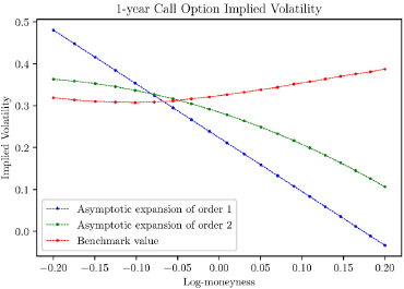
Figure 10.2. An example of the asymptotic expansions of orders 1 and 2 of the implied volatility, and the benchmark value for a call option with a maturity of 1 year
10.4. Calibration using the asymptotic expansions
The numerical study in the previous section gives a base for the calibration. We know now for which range of log-moneyness and maturities the first- and second-order expansions can be used as calibration formulas.
10.4.1. A partial calibration procedure
We propose a simple partial calibration procedure for some model parameters or some grouped expressions of parameters. By saying partial calibration, we mean that only a part of the original model parameters or a grouped form of them will be calibrated. If a full calibration is desired, we can use the results from the partial calibration as inputs for the final local optimization over all model parameters. For this step, we can use the second-order implied volatility and market options with a suitable range of maturities and strikes as given in the previous section. As this step of full calibration is a standard procedure, we will not discuss it here.
To explain the partial calibration procedure, recall the form of the asymptotic expansion of order 1 of implied volatility:
and the form of the asymptotic expansion of order 2 of the implied volatility:
Note from these forms that by setting in equation [10.3]:
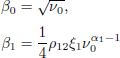
and in equation [10.4]:
the calibration formulas become:
The calibration goes as follows. First, consider the asymptotic expansion of order 1 of the implied volatility in the form given by equation [10.7]. Looking at the log-moneyness k − x0 as the independent variable, and the σ1 as a dependent variable, the form can be seen as a simple linear regression model. The numerical study suggests that the optimal choice of log-moneyness to fit the model would be between −0.1 and 0.07, using 30 days options. By doing so, the estimate of the intercept β0 leads to ![]() , and the estimate of the slope β1 leads to
, and the estimate of the slope β1 leads to ![]() . In combination, thos two quantities finally yield values for ν0 and the product ρ12ξ1.
. In combination, thos two quantities finally yield values for ν0 and the product ρ12ξ1.
Next, from equation [10.8], looking at T − t as the independent variable and σ2 as the dependent variable, a simple linear regression can be fitted. However, to get the required estimates, a previous discussion should be used in combination with equations [10.5] and [10.6]. That is, as the asymptotic expansion of order 1 of the implied volatility leads to ν0 and ρ12ξ1, this can be used in equations [10.5] and [10.6] to eliminate those parameters. Next, using at-the-money options, only part of equation [10.6] of the interest is the product ![]() that may be obtained from the slope.
that may be obtained from the slope.
To get the calibrated values using equation [10.4], at-the-money 30 days to 1 year options are used in combination with calibrated values ν0, ρ12ξ1, obtained from equation [10.3] as explained.
Therefore, this procedure gives calibrated values of ![]() . It is worth reiterating that these values may be used as an intermediate result for a local optimization procedure on a full calibration such that the difference between the model implied volatilizes and market implied volatilities are minimized.
. It is worth reiterating that these values may be used as an intermediate result for a local optimization procedure on a full calibration such that the difference between the model implied volatilizes and market implied volatilities are minimized.
10.4.2. Calibration to synthetic and market data
To compare the calibrated and true parameter values, a good way to start is by generating an implied surface using the Monte Carlo simulation with a known set of parameters and applying the calibration procedure. To do so, the Gatheral model with parameters given in Table 10.1 and a fixed value of α1 = α2 = 0.94 is used. The synthetic data is generated for options with log-moneyness from −0.2 to 0.2, and maturities from 30 days to 2 years, but, as discussed previously in the calibration procedure, only the part of options with suitable log-moneyness and maturities are used.
As expected, the calibration gives close-to-true values. Table 10.2 shows that the difference between true and calibrated values is fairly small.
Table 10.2. Result of calibration using synthetic data
| Parameter/initial value | True value | Calibrated |
| ν0 | 0.050 | 0.049 |
| ρ12ξ1 | −2.8500 | −2.6424 |
| −0.055 | −0.031 |
Before moving to the calibration of the real market data, a short description of the dataset follows. It consists of daily implied volatility surfaces calculated and interpolated from the traded call options on ABB stock and on Eurostock 50 Index, in Nasdaqomx Nordic Exchange and Eurex, respectively. The dataset is processed from the data provided by the company OptionMetrics LLC. The period is from November 2019 to November 2020. That is, it starts before the Covid-19 pandemic, which could be interesting. There are 10 time-to-maturities, 30, 60, 91, 122, 152, 182, 273, 365, 547 and 730 calendar days, There are also 13 implied exercise prices obtained from the well-known Greek Deltas (0.20 + 0.05n, n = 0, 1, 2,...,12). For this study, only options with maturities from 30 days to 1 year with a suitable range of log-moneyness are of interest. While using the first-order expansion, we take 30-day options with a range of log-moneyness from −0.1 to 0.07. We use at-the-money (or closely at-the-money) options with maturities from 30 days to 1 year for the second-order expansion.
For simplicity, we calibrate the special case of Double Lognormal model, i.e. we set α1 = α2 = 1.
Applying the calibration procedure to the real market data, Figures 10.3 and 10.4 show calibrated daily values of the volatility process of the ABB stock and Eurostock 50 Index, respectively. On both figures, it is clear that the pandemic had a great impact on the volatility, in the middle of March. This period is when Covid-19 started spreading in Europe, and high volatility was expected.
Figures 10.5 and 10.6 show calibrated daily values of the product of the correlation ρ12 and ξ1 of the ABB stock and Eurostock 50 Index, respectively. Because ξ1 is assumed to be positive, and the realistic situation suggests that ρ12 should be negative, the product should be negative too. This can be seen in Figure 10.5. Besides this, the product should be constant if the Double Lognormal model is a representation of the market. However, in Figure 10.6, it can be seen that there are some extremely positive values. As the situation is severe, due to Covid-19, a calibration should be done more often during this period to avoid getting unrealistic values. Again, in both cases, the impact of the pandemic is obvious.
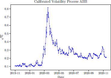
Figure 10.3. Calibrated daily values for the daily volatility  using ABB stock data
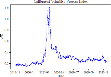
Figure 10.4. Calibrated daily values for the daily volatility using Eurostock 50 Index data
To calibrate daily values for the product of reversion rate κ1 and difference ![]() ,
, ![]() , as mentioned, a linear regression of implied volatilities against a range of time-to-maturities for at-the-money options was used. Figures 10.7 and 10.8 show values obtained from the calibration for the ABB stock and Eurostock 50 Index, respectively. It seems like the pandemic had more impact on the ABB stock in this case. During the middle of March, the effect of the Covid-19 pandemic was undoubtedly the largest.
, as mentioned, a linear regression of implied volatilities against a range of time-to-maturities for at-the-money options was used. Figures 10.7 and 10.8 show values obtained from the calibration for the ABB stock and Eurostock 50 Index, respectively. It seems like the pandemic had more impact on the ABB stock in this case. During the middle of March, the effect of the Covid-19 pandemic was undoubtedly the largest.
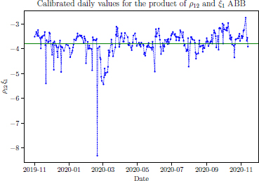
Figure 10.5. Calibrated daily values for the product of ρ12 and ξ1, ρ12ξ1, using ABB stock data
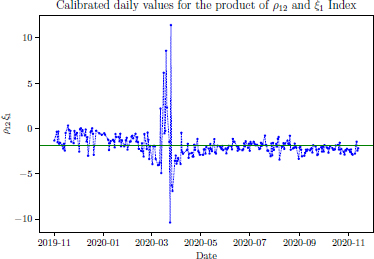
Figure 10.6. Calibrated daily values for the product of ρ12 and ξ1, ρ12 ξ1, using Eurostock 50 Index data
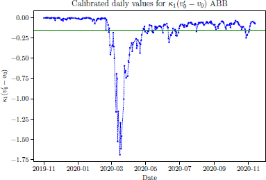
Figure 10.7. Calibrated daily values for the product  using ABB stock data
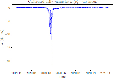
Figure 10.8. Calibrated daily values for the product using Eurostock 50 Index data
10.5. Conclusion and future work
We have investigated the performance of the first- and second-order implied volatility expansions under the Gatheral model and concluded that the first-order expansion gives a plausible approximation when the maturity is as short as 30 days.
In contrast, the second-order expansion yields good approximations for maturity up to 1 year. Both expansions work well only for a range of values of log-moneyness.
A simple partial calibration procedure was presented, taking advantage of a simple polynomial form of these expansions as functions of maturities and log-moneyness. In implementing our calibration procedure, note that the effect of the Covid-19 pandemic on the model calibration is high. It can especially be noted during the middle of March, when the effect is the largest. Particular attention should be paid to the calibration when the market is undergoing a similar crisis.
In future work, the performance of the third-order asymptotic expansion for implied volatility should be studied and compared to the second-order expansion. A full calibration to the market data can also be done.
10.6. References
Albuhayri, M., Malyarenko, A., Silvestrov, S., Ni, Y., Engström, C., Tewolde, F., Zhang, J. (2021). Asymptotics of implied volatility in the gatheral double stochastic volatility model. In Applied Modeling Techniques and Data Analysis 2, Dimotikalis, Y., Karagrigoriou, A., Parpoula, C., Skiadas, C.H. (eds). ISTE Ltd, London, and John Wiley & Sons, New York.
Bayer, C., Gatheral, J., Karlsmark, M. (2013). Fast Ninomiya–Victoir calibration of the double-mean-reverting model. Quantitative Finance, 13(11), 1813–1829.
Berestycki, H., Busca, J., Florent, I. (2002). Asymptotics and calibration of local volatility models. Quantitative Finance, 2(1), 61–69.
Dupire, B. (1997). Pricing and hedging with smiles. In Mathematics of Derivative Securities, Dempster, M.A.H. and Pliska, S.R. (eds). Cambridge University Press, Cambridge.
Fouque, J.P., Papanicolaou, G., Sircar, R., Sølna, K. (2011). Multiscale Stochastic Volatility for Equity, Interest Rate, and Credit Derivatives. Cambridge University Press, Cambridge.
Gatheral, J. (2008). Consistent modeling of SPX and VIX options. Paper presented at The Fifth World Congress of the Bachelier Finance Society, London, 18 July 2008.
Hilpisch, Y. (2019). Derivatives Analytics with Python: Data Analysis, Models, Simulation, Calibration and Hedging. John Wiley & Sons, New York.
Pagliarani, S. and Pascucci, A. (2017). The exact Taylor formula of the implied volatility. Finance and Stochastics, 21(3), 661–718.
Chapter written by Marko DIMITROV, Mohammed ALBUHAYRI, Ying NI and Anatoliy MALYARENKO.