
18
Data Analysis based on Entropies and Measures of Divergence
In this chapter, we discuss entropies and measures of divergence which are extensively used in data analysis and statistical inference. Tests of goodness of fit are reviewed and their asymptotic theory is discussed. Simulation studies are undertaken for comparing their performance capabilities.
18.1. Introduction
Measures of divergence are powerful statistical tools directly related to statistical inference, including robustness, with diverse applicability (see, for example, Papaioannou 1985; Basu et al. 2011; Ghosh et al. 2013). Indeed, on one hand, they can be used for estimation purposes with the classical example, the well-known maximum likelihood estimator (MLE) which is the result of the implementation of the famous Kullback–Leibler measure. On the other hand, measures are applicable in tests of fit to quantify the degree of agreement between the distribution of an observed random sample and a theoretical, hypothesized distribution. The problem of goodness of fit (gof) to any distribution on the real line is frequently treated by partitioning the range of data in a number of disjoint intervals. In all cases, a test statistic is compared against a known critical value to accept or reject the hypothesis that the sample is from the postulated distribution. Over the years, numerous non-parametric gof methods including the chi-squared test and various empirical distribution function (edf) tests (D’Agostino and Stephens 1986) have been developed. At the same time, measures of entropy, divergence and information are quite popular in goodness-of-fit tests. Over the years, several measures have been suggested to reflect the fact that some probability distributions are closer together than others. Many of the currently used tests, such as the likelihood ratio, the chi-squared, the score and Wald tests are defined in terms of appropriate measures.
In this chapter, we provide a comprehensive review on entropies and distance measures and their use in inferential statistics. Section 18.2 is devoted to a brief literature review on entropies and divergence measures, and Section 18.3 presents the main results on tests of fit. Section 18.4 through extensive simulations explores the performance of a recently proposed double index test of fit in contingency tables.
18.2. Divergence measures
Measures of information are powerful statistical tools with diverse applicability. In this section, we will focus on a specific type of information measure, known as measures of discrepancy (distance or divergence) between two variables X and Y with pdfs f and g. Furthermore, we will explore ways to measure the discrepancy between (i) the distribution of X as deduced from an available set of data and (ii) the distribution of X as compared with a hypothesized distribution believed to be the generating mechanism that produced the set of data at hand.
For historical reasons, we present first Shannon’s entropy (Shannon 1948) given by
where X is a random variable with density function f(x) and μ is a probability measure on ℝ. The development of the concept of entropy started in the 19th century in the field of physics and in particular in describing thermodynamics processes, but the development of the statistical description of entropy by Boltzmann led to a strong resistance by many. Shannon’s entropy was introduced and used during World War II in Communication Engineering. Shannon derived the discrete version of IS(f ), where f is a probability mass function and named it entropy because of its similarity to thermodynamics entropy. The continuous version was defined by analogy and it is called differential entropy (Cover and Thomas 2006). For a finite number of points, Shannon’s entropy measures the expected information of a signal provided without noise from a source X with density f (x) and is related to the Kullback–Leibler divergence (Kullback and Leibler 1951) through the following expression:
where h is the density of the uniform distribution and the Kullback–Leibler divergence between two densities f(x) and g(x) is given by
Many generalizations of Shannon’s entropy were hereupon introduced. Rényi’s (1963) entropy as extended by Liese and Vajda (1987) is given by
For more details about entropy measures, the reader is referred to Mathai and Rathie (1975) and Nadarajah and Zografos (2003).
A measure of divergence is used as a way to evaluate the distance (divergence) between any two functions f and g associated with the variables X and Y. Among the most popular measures of divergence are the Kullback–Leibler measure of divergence given in [18.1] and Csiszar’s ϕ-divergence family of measures (Csiszar 1963; Ali and Silvey 1966) given by
where ϕ is a convex function on [0, ∞) such that ϕ (1) = ϕ’ (1) = 0 and ϕ″ (1) ≠ 0. We also assume the conventions 0ϕ (0/0) = 0 and ![]() . The class of Csiszar’s measures includes a number of widely used measures that can be recovered for appropriate choices of the function ϕ. When the function ϕ is defined as
. The class of Csiszar’s measures includes a number of widely used measures that can be recovered for appropriate choices of the function ϕ. When the function ϕ is defined as
then the above measure reduces to the Kullback–Leibler measure given in [18.1]. If
Csiszar’s measure yields Pearson’s chi-square divergence (also known as Kagan’s divergence; Kagan (1963)). If
or
we obtain the Cressie and Read power divergence (Cressie and Read 1984), λ ≠ 0, −1.
Another function usually considered in practice is
which is associated with the BHHJ power divergence (Basu et al. 1998) and is a member of the BHHJ family of divergence measures proposed by Mattheou et al. (2009), which depends on a general convex function Φ and a positive index a and is given by
where μ represents the Lebesgue measure and Φ* is the class of all convex functions Φ on [0, ∞) such that Φ (1) = Φ′ (1) = 0 and Φ″ (1) ≠ 0. We also assume the conventions 0Φ (0/0) = 0 and ![]() .
.
Appropriately chosen functions Φ(·) give rise to special measures mentioned above, while for α = 0, the BHHJ family reduces to Csiszar’s family. Expression [18.7] covers not only the continuous case but also the discrete one where the measure μ is a counting measure. Indeed, for the discrete case, the divergence in [18.7] is meaningful for probability mass functions f and g whose support is a subset of the support Sμ, finite or countable, of the counting measure μ that satisfies μ (x) = 1 for x ∈ Sμ and 0 otherwise. The discrete version of the Φ−family of divergence measures is presented in the definition below.
DEFINITION.– For two discrete distributions P = (p1,... , pm)′ and Q = (q1,... , qm)′ with sample space Ω = {x : p(x) q(x) > 0}, where p(x) and q(x) are the probability mass functions of the two distributions, the discrete version of the Φ−family of divergence measures with a general function Φ ∈ Φ∗ and a > 0 is given by
For Φ having the special form given in [18.6], we obtain the BHHJ measure (Basu et al. 1998) which was proposed for the development of a minimum divergence estimating method for robust parameter estimation. Observe that for Φ (u) = φ (u) ∈ Φ0 and a = 0, the family reduces to Csiszár’s φ−divergence family of measures, while for a = 0 and for Φ (u) = ϕλ(u) as in [18.5], it reduces to the Cressie and Read power divergence measure. Other important special cases of the Φ−divergence family are those for which the function Φ(u) takes the form
and
It is easy to see that for a → 0, the measures Φa(·) and ![]() reduce to the KL measure.
reduce to the KL measure.
More examples of φ functions are given in Arndt (2001) and Pardo (2006). For more details on divergence measures, see Cavanaugh (2004), Toma (2009) and Toma and Broniatowski (2011). Specifically, for robust inference based on divergence measures, see Basu et al. (2011) and a paper by Patra et al. (2013) on the power divergence and the density power divergence families. The descritized version of measures has been given considerable attention over the years, with some representative works being by Zografos et al. (1986) and Papaioannou et al. (1994).
18.3. Tests of fit based on Φ−divergence measures
In this section, we discuss the problem of goodness-of-fit tests via divergence measures. Assume that X1, ..., Xn are i.i.d. random variables with common distribution function (d.f.) F . Given some specified d.f. F0, the classical goodness-of-fit problem is concerned with testing the simple null hypothesis H0 : F = F0. This problem is frequently treated by partitioning the range of data in m disjoint intervals and by testing a hypothesis based upon the vector of parameters of a multinomial distribution.
Let P = {Ei}i=1,..., m be a partition of the real line ℝ in m intervals. Let p = (p1,..., pm)′ and p0 = (p10,..., pm0)′ be the true and the hypothesized probabilities of the intervals Ei, i = 1,..., m, respectively, in such a way that pi = PF (Ei), i = 1,... ,m and ![]() .
.
Let Y1,..., Yn be a random sample from F and let ![]() with
with ![]() , where
, where
and ![]() with
with ![]() be the MLE of pi.
be the MLE of pi.
Although the above simple null hypothesis frequently appears in practice, it is common to test the composite null hypothesis that the unknown distribution belongs to a parametric family {F0}0 ∈Θ, where Θ is an open subset in Rk. In this case, we can again consider a partition of the original sample space with the probabilities of the elements of the partition depending on the unknown k−dimensional parameter θ. Then, the hypothesis can be tested by the hypotheses
where θ0 is the true value of the k-dimensional parameter under the null model and p0(θ0) = (p10(θ0),..., pm0(θ0))′. Pearson encountered this problem in the well-known chi-square test statistic and suggested the use of a consistent estimator for the unknown parameter. He further claimed that the asymptotic distribution of the resulting test statistic, under the null hypothesis, is a chi-square random variable with m degrees of freedom. Later, for the same test, Fisher (1924) established that the correct distribution has m − 1 degrees of freedom. The result was later discussed by Neyman (1949) and recently by Menendez et al. (2001). In this case, since the null distribution depends on the unknown parameter θ, a consistent estimator of θ is required.
The partition of the data range is a delicate matter since it is frequently associated with the loss of information. For a thorough investigation on the issue, the interested reader is referred to the works by Ferentinos and Papaioannou (1979, 1983).
For testing the above null hypotheses, the most commonly used test statistics are Pearson’s or the chi-squared test statistic and the likelihood ratio test statistic which are both special cases of the family of power-divergence test statistics (CR test) which was introduced by Cressie and Read (1984), is based on the measure given in [18.5] and is given by
where λ ≠ −1, 0, −∞ < λ < ∞, ![]() , and
, and ![]() is a consistent estimator of θ. Particular values of λ in [18.12] correspond to well-known test statistics: chi-squared test statistic (λ = 1), likelihood ratio test statistic (λ → 0), Freeman–Tukey test statistic (λ = −1/2), minimum discrimination information statistic (Gokhale and Kullback 1978; Kullback 1985) (λ → −1), modified chi-squared test statistic (Neyman 1949) (λ = −2) and Cressie–Read test statistic (λ = 2/3).
is a consistent estimator of θ. Particular values of λ in [18.12] correspond to well-known test statistics: chi-squared test statistic (λ = 1), likelihood ratio test statistic (λ → 0), Freeman–Tukey test statistic (λ = −1/2), minimum discrimination information statistic (Gokhale and Kullback 1978; Kullback 1985) (λ → −1), modified chi-squared test statistic (Neyman 1949) (λ = −2) and Cressie–Read test statistic (λ = 2/3).
Although the power-divergence test statistics yield an important family of tests of fit, it is possible to consider the more general Csiszar’s family of φ − divergence test statistics for testing [18.11] which contains [18.12] as a particular case is based on the discrete form of [18.2] and is defined by
with φ(x) a convex, twice continuously differentiable function for x > 0 such that φ″ (1) ≠ 0.
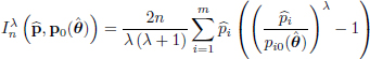
The above family of tests was generalized by Mattheou and Karagrigoriou (2010) to the following Φ−family of tests which is based on the Φ−divergence measure given in [18.8]:
Cressie and Read (1984) obtained the asymptotic distribution of the power-divergence test statistic ![]() given in [18.12], Zografos et al. (1990) extended the result to the family
given in [18.12], Zografos et al. (1990) extended the result to the family ![]() for a = 0 and Φ = φ ∈ Φ0 and Mattheou and Karagrigoriou (2010) extended the result to cover any function Φ ∈ Φ*:
for a = 0 and Φ = φ ∈ Φ0 and Mattheou and Karagrigoriou (2010) extended the result to cover any function Φ ∈ Φ*:
THEOREM 18.1.– (Cressie and Read 1984). Under the null hypothesis H0 : p = p0 = (p10,..., pm0)′, the asymptotic distribution of the Cressie and Read divergence test statistic, ![]() , is chi-square with m − 1 degrees of freedom:
, is chi-square with m − 1 degrees of freedom:
THEOREM 18.2.– (Zografos et al. 1990). Under the null hypothesis H0 : p = p0 = (p10,..., pm0)′, the asymptotic distribution of the φ − divergence test statistic, ![]() , is chi-square with m − 1 degrees of freedom:
, is chi-square with m − 1 degrees of freedom:
THEOREM 18.3.– (Mattheou and Karagrigoriou 2010). Under the composite null hypothesis H0 : p = p0(θ0), the asymptotic distribution of the Φ−divergence test statistic, ![]() divided by a constant c, is chi-square with m − 1 degrees of
divided by a constant c, is chi-square with m − 1 degrees of
where
and ![]() a consistent estimator of θ.
a consistent estimator of θ.
For the case of the simple null hypothesis, the theorem is adjusted accordingly and the asymptotic distribution is therefore chi-square with m − 1 degrees of freedom. For the fixed alternative hypothesis, the power is given in the theorem below:
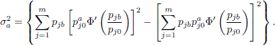
THEOREM 18.4.– The power of the test H0 : pi = pi0 vs Ha : pi = pib, i = 1, ..., m using the test statistic [18.15] with ![]() is approximately equal to:
is approximately equal to:
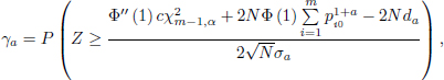
where Z a standard normal random variable, and
It is known that it is not always possible to determine the asymptotic distribution under any alternative. Here, we will provide the asymptotic distribution under contiguous alternatives. Suppose that the simple null hypothesis indicates that pi = pi0, i = 1, 2,... ,m when in fact it is pi = pib, ∀i. As is well known, if pi0 and pib are fixed, then as n tends to infinity, the power of the test tends to 1. In order to examine the situation when the power is not close to 1, we must make it continually harder for the test as n increases. This can be done by allowing the alternative hypothesis steadily closer to the null hypothesis. As a result, we define a sequence of alternative hypotheses as follows
where pn = (p1n,... , pmn)′ and d = (d1,..., dm)′ is a fixed vector such that ![]() . This hypothesis is known as the Pitman (local) alternative or local contiguous alternative to the null hypothesis H0 : p = p0. Observe that as n tends to infinity, the local contiguous alternative converges to the null hypothesis at the rate O(n−1/2).
. This hypothesis is known as the Pitman (local) alternative or local contiguous alternative to the null hypothesis H0 : p = p0. Observe that as n tends to infinity, the local contiguous alternative converges to the null hypothesis at the rate O(n−1/2).
The following theorem by Mattheou and Karagrigoriou (2010) provides the asymptotic distribution under contiguous alternatives.
THEOREM 18.5.– Under the contiguous alternative hypothesis given in [18.19], the asymptotic distribution of the Φ−divergence test statistic, ![]() divided by a constant c, is a non-central chi-square with m − 1 degrees of freedom:
divided by a constant c, is a non-central chi-square with m − 1 degrees of freedom:
where ![]() and non-centrality parameter
and non-centrality parameter ![]() .
.
Due to the above theorems, the power of the test under the fixed alternative hypothesis H1 : pi = pib and the local contiguous alternative hypotheses [18.19]
can be easily obtained. For the case of the local contiguous alternative hypotheses, the power is given by
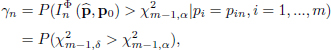
Where ![]() is the α−percentile of the
is the α−percentile of the ![]() distribution.
distribution.
We close this section with a short discussion about the estimation of the unknown parameter θ which is a classic inferential problem. Optimal estimating approaches, like the maximum likelihood estimation, are available in the literature (e.g. Papaioannou et al. 2007). Here, we focus on the parameter estimator under the composite hypothesis. Although the traditional MLE can be evaluated and implemented, we may alternatively consider a wider class of estimators, known as Φ−divergence estimators. More specifically, the minimum Φ−divergence estimator of θ is any ![]() satisfying
satisfying
for a function Φ ∈ Φ* and with ![]() . Obviously, the resulting estimator depends on the Φ-function chosen. Observe that for Φ as in [18.6] or [18.10] and for a → 0, the resulting estimator is the usual MLE for the grouped data. It should be pointed out that the function Φ used for the Φ−divergence estimator
. Obviously, the resulting estimator depends on the Φ-function chosen. Observe that for Φ as in [18.6] or [18.10] and for a → 0, the resulting estimator is the usual MLE for the grouped data. It should be pointed out that the function Φ used for the Φ−divergence estimator ![]() does not necessarily coincide with the Φ-function used for the test statistic which, in general, is written as
does not necessarily coincide with the Φ-function used for the test statistic which, in general, is written as
where
for two, not necessarily different functions Φ1 & Φ2 ∈ Φ*. Finally, note that such a type of estimator has been thoroughly investigated and their asymptotic theory has been presented in Meselidis and Karagrigoriou (2020). Indeed, the innovative idea behind the proposal by Meselidis and Karagrigoriou (2020) is the duality in choosing among the members of the general class of divergences, one for estimating and one for testing purposes which may not necessarily be the same. In that sense, the divergence test statistic given in [18.20] offers the greatest possible range of options both for the strictly convex function Φ and the indicator value α ∈ R. More specifically, if a parameter θ needs to be estimated, then a function Φ, say Φ2, and an index α, say α2, are used for that purpose and then we proceed with the distance and the testing problem using a function Φ, say Φ1, and an index α, say α1, which, in general, can be different from those used for the estimation problem. The resulting divergence is given in [18.20] and [18.21], where ![]() is the minimum (Φ2, α2) divergence estimator which is allowed to be obtained even under restrictions, say c(θ) = 0.
is the minimum (Φ2, α2) divergence estimator which is allowed to be obtained even under restrictions, say c(θ) = 0.
18.4. Simulations
The problem of contingency tables or cross-tabulations and their statistical analysis based on measures of divergence always attracts the attention of researchers with a plethora of important contributions (see, for example, Kateri et al. 1996; Kateri and Papaioannou 1997, 2007). Such problems though are often associated with two serious issues that frequently appear in practice and considerably affect both estimating and testing procedures, namely censoring and contamination often encountered among other fields, in survival analysis (see Basu et al. 2006; Vonta and Karagrigoriou 2010; Sachlas and Papaioannou 2014). For an extensive overview of such issues and their handling, please refer to Tsairidis et al. (1996, 2001). The emphasis in this section is on contamination. More specifically, in order to attain a better insight of the behavior of the proposed divergences used both for estimation and testing purposes, we proceed further with a simulation study. The null hypothesis considered focuses on the Gamma distribution with a shape parameter equal to 1, denoted by Γ(1). On the other hand, as alternative hypotheses, we have used Gamma distributions with shape parameters equal to 1.5, 4.0 and 10.0 denoted by Γ(1.5), Γ(4) and Γ(10), respectively. In every case, the scale parameter is chosen to be equal to 1 due to the fact that the distribution is scale invariant.
The study is implemented not only for the regular case but also for cases where the data set is contaminated. In this regard, we define α as the contamination level with α ∈ [0, 1]. Thus, the data generating distribution has the form (1 − α)Γd + αΓc, where Γd is the dominant and Γc the contaminant Gamma distribution. Note that the contamination level used is taken to be equal to 0.075. Thus, for the examination of estimators and test statistics in terms of size of the test (α), we contaminate the null distribution with observations from the alternative hypotheses and vice versa for the examination of tests in terms of power (γ). Furthermore, for the implementation, we have considered a large sample size, n = 200 and N = 100000 repetitions of the experiment, while for the partition of the data range, we use ![]() equiprobable intervals, where the ⎡·⎤ operator returns the least integer which is greater than or equal to its argument.
equiprobable intervals, where the ⎡·⎤ operator returns the least integer which is greater than or equal to its argument.
As classical minimum divergence estimators, we use those that can be derived from the Cressie–Read family for λ = −2, −1, −1/2, 0, 2/3, 1 which are known as the minimum modified chi-squared (![]() ), discrimination information (
), discrimination information (![]() ), Freeman–Tukey (
), Freeman–Tukey (![]() ), likelihood ratio (
), likelihood ratio (![]() ), Cressie–Read (
), Cressie–Read (![]() ) and chi-squared (
) and chi-squared (![]() ) estimators. On the other hand, the proposed BHHJ family of estimators (
) estimators. On the other hand, the proposed BHHJ family of estimators (![]() ) is applied for 13 values of the parameters α2 = 10−7, 0.01, 0.05, 0.10...(0.10)...1.00 and Φ2 as in [18.6]. Furthermore, we have included in our analysis not only the L2-distance estimator (
) is applied for 13 values of the parameters α2 = 10−7, 0.01, 0.05, 0.10...(0.10)...1.00 and Φ2 as in [18.6]. Furthermore, we have included in our analysis not only the L2-distance estimator (![]() ) which along with the likelihood ratio serve as benchmark estimators (divergences in general) since they are equivalent with the BHHJ family for α = 1 and α → 0, respectively, but also the MLE (
) which along with the likelihood ratio serve as benchmark estimators (divergences in general) since they are equivalent with the BHHJ family for α = 1 and α → 0, respectively, but also the MLE (![]() ) based on the ungrouped data.
) based on the ungrouped data.
In reference to the test statistics, we proceed in a similar manner and retrieve from the Cressie–Read family the classical modified chi-squared MCS (![]() ), minimum discrimination information MDI(
), minimum discrimination information MDI(![]() ), Freeman–Tukey FT (
), Freeman–Tukey FT (![]() ), likelihood ratio
), likelihood ratio ![]() , Cressie–Read
, Cressie–Read ![]() and Pearson’s chi-squared
and Pearson’s chi-squared ![]() test statistics along with the proposed
test statistics along with the proposed ![]() for α1 = 10−7, 0.01, 0.05, 0.10...(0.10)...1.00 and Φ1 as in [18.6].
for α1 = 10−7, 0.01, 0.05, 0.10...(0.10)...1.00 and Φ1 as in [18.6].
The examination of the behavior of the minimum divergence estimators is based on the mean-squared error (MSE) given by
with ![]() being the minimum divergence estimator based on any I divergence for the lth sample.
being the minimum divergence estimator based on any I divergence for the lth sample.
Figure 18.1 presents the MSE for the four cases which are associated with no contamination and contamination from the three alternative distributions. The minimum divergence estimators are displayed in acceding order following a counterclockwise direction according to the case where the contaminant distribution lies far from the null, i.e. when the data are generated from 0.925Γ(1) + 0.075Γ(10). Results indicate that in terms of MSE, estimators that can be derived from the Cressie–Read family with λ ≥ 0 along with those that can be derived from the BHHJ family with small values of α2 have better performance for the no contamination case and when the contaminant distribution is close to the null (Figures 18.1a and 18.1b). Note that in these two cases, (![]() ) has the best performance among all competing estimators. On the contrary, when the contaminant distribution departs further from the null (Figures 18.1c and 18.1d), estimators from the BHHJ family with larger values of α2 and those from the Cressie–Read family with negative values of λ appear to behave better while the worst results arise for the
) has the best performance among all competing estimators. On the contrary, when the contaminant distribution departs further from the null (Figures 18.1c and 18.1d), estimators from the BHHJ family with larger values of α2 and those from the Cressie–Read family with negative values of λ appear to behave better while the worst results arise for the ![]() . In addition, Figure 18.1 reveals the robustness aspect of the BHHJ and the Cressie–Read estimators since it is apparent that in the presence of contamination the larger the value of the index α2 and the smaller the value of the parameter λ the smaller the MSE. Finally, note that in every case, the MSE of
. In addition, Figure 18.1 reveals the robustness aspect of the BHHJ and the Cressie–Read estimators since it is apparent that in the presence of contamination the larger the value of the index α2 and the smaller the value of the parameter λ the smaller the MSE. Finally, note that in every case, the MSE of ![]() lies between the MSEs of the
lies between the MSEs of the ![]() and the
and the ![]() . We should state here that for presentation purposes, the MSE has been multiplied by 100. For more information about robust estimation for grouped data, refer to Basu et al. (1997), Victoria-Feser and Ronchetti (1997), Lin and He (2006) and Toma and Browniatowski (2011), while for the mathematical connection of the BHHJ and Cressie–Read families, refer to Patra et al. (2013).
. We should state here that for presentation purposes, the MSE has been multiplied by 100. For more information about robust estimation for grouped data, refer to Basu et al. (1997), Victoria-Feser and Ronchetti (1997), Lin and He (2006) and Toma and Browniatowski (2011), while for the mathematical connection of the BHHJ and Cressie–Read families, refer to Patra et al. (2013).
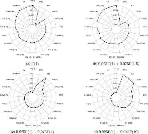
Figure 18.1. MSE (×100) for the four cases of contamination regarding the tests that can be derived both from the BHHJ and Cressie–Read families
Under the setup of this study, we have m = 15 probabilities of the multinomial model and k = 1 unknown parameters to estimate; thus, the critical values used are the asymptotic critical values based on the asymptotic distribution ![]() with
with ![]() , being a generalization of [18.17], for the BHHJ family of test statistics, and the
, being a generalization of [18.17], for the BHHJ family of test statistics, and the ![]() for the classical test statistics that can be derived from the Cressie–Read family, with a nominal level equal to 0.05.
for the classical test statistics that can be derived from the Cressie–Read family, with a nominal level equal to 0.05.
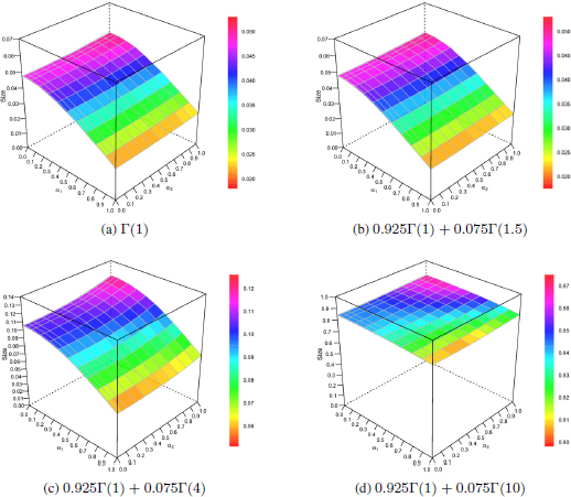
Figure 18.2. Size for the four contamination cases regarding the tests that can be derived from the BHHJ family. For a color version of this figure, see www.iste.co.uk/zafeiris/data1.zip
In Figure 18.2, we examine under the four aforementioned cases the behavior of the BHHJ test statistics in terms of size for various values of the indices α1 and α2, while in Table 18.1, the behavior of the classical tests is presented. In general, we can see that as the index α1 increases, the size decreases, while as the index α2 increases, the size increases as well. Furthermore, we can observe that in the case where the contaminant distribution lies far from the null (Figure 18.2d), the size becomes very large, indicating the disastrous effect imposed from the contaminant distribution to all BHHJ test statistics. This disastrous effect is also apparent in the classical test statistics. In the case where the contaminant distribution is the Γ(4) (Figure 18.2c), the BHHJ family of tests discounts the effect of contamination for values of α1 ≥ 0.8, while the classical tests are largely affected by the contamination once again. Finally, for the no contamination and contamination from the Γ(1.5), we can derive the following conclusions about the behavior of the tests. Regarding the BHHJ family (Figures 18.2a and 18.2b), we can observe that the larger the value of α1, the more conservative the test is, while the best performance appears for α1 ≤ 0.10 and α2 ≥ 0.50. With respect to the classical tests, ![]() ,
, ![]() and
and ![]() appear to be conservative, while CS(
appear to be conservative, while CS(![]() ) and CS(
) and CS(![]() ) appear to be liberal. Note that in terms of size, LR
) appear to be liberal. Note that in terms of size, LR![]() appears to have the best performance among all classical test statistics.
appears to have the best performance among all classical test statistics.
Table 18.1. Size for the four contamination cases regarding the classical tests that can be derived from the Cressie–Read family
| Data distribution | FT | CR | CS | LR | MDI | MCS |
| Γ(1) | 0.04028 | 0.06538 | 0.07841 | 0.04744 | 0.03783 | 0.04263 |
| 0.925Γ(1) + 0.075Γ(1.5) | 0.03943 | 0.06759 | 0.08195 | 0.04775 | 0.03659 | 0.04072 |
| 0.925Γ(1) + 0.075Γ(4) | 0.09546 | 0.12762 | 0.14392 | 0.10539 | 0.09063 | 0.09521 |
| 0.925Γ(1) + 0.075Γ(10) | 0.83558 | 0.85420 | 0.85953 | 0.85953 | 0.82183 | 0.68850 |
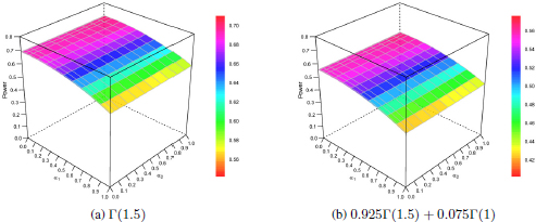
Figure 18.3. Power for the no contamination and contamination from Γ(1) cases regarding the tests that can be derived from the BHHJ family. For a color version of this figure, see www.iste.co.uk/zafeiris/data1.zip
Table 18.2. Power for the no contamination and contamination from Γ(1) cases regarding the classical tests that can be derived from the Cressie–Read family
| Data distribution | FT | CR | CS | LR | MDI | MCS |
| Γ(1.5) | 0.69412 | 0.69911 | 0.70887 | 0.69061 | 0.70568 | 0.74808 |
| 0.925Γ(1.5) + 0.075Γ(1) | 0.55308 | 0.57515 | 0.59049 | 0.55571 | 0.56224 | 0.60448 |
In terms of power, results are presented in Figure 18.3 and Table 18.2 for the BHHJ and classical tests, respectively. Note that we only present results that are associated with the Γ(1.5) alternative since in every other case the power reaches the highest level 1 for all tests. As a general conclusion, we can state that the contamination affects the performance of all tests by notably downgrading their power. Concerning the BHHJ tests, the best results appear for small values of α1 and large values of α2, while the classical modified chi-squared test statistic, ![]() , has the best performance among all classical tests.
, has the best performance among all classical tests.
Based on the preceding analysis, we proceed further with the comparison of the tests. Beyond the classical ones, we choose the following four test statistics from the BHHJ family ![]() ,
, ![]() and
and ![]() ). In order to derive solid conclusions about the behavior of the test statistics in terms of size, we consider Dale’s criterion (Dale 1986) which involves the following inequality:
). In order to derive solid conclusions about the behavior of the test statistics in terms of size, we consider Dale’s criterion (Dale 1986) which involves the following inequality:
where logit(p) = log(p/(1 − p)), while ![]() and α are the exact simulated and nominal sizes, respectively. When [18.22] is satisfied with d = 0.35, the exact simulated size is considered to be close to the nominal size. For α = 0.05, the exact simulated size is close to the nominal if
and α are the exact simulated and nominal sizes, respectively. When [18.22] is satisfied with d = 0.35, the exact simulated size is considered to be close to the nominal size. For α = 0.05, the exact simulated size is close to the nominal if ![]() . This criterion has been used previously by Pardo (2010) and Batsidis et al. (2016). We apply the criterion not only for α = 0.05 but also for a range of nominal sizes that are of interest, namely α ∈ [0, 0.1].
. This criterion has been used previously by Pardo (2010) and Batsidis et al. (2016). We apply the criterion not only for α = 0.05 but also for a range of nominal sizes that are of interest, namely α ∈ [0, 0.1].
Results are presented in Figure 18.4, where the dashed line refers to the situation where the exact simulated equals the nominal size; thus, lines that lie above this reference line refer to liberal, while those that lie below refer to conservative test statistics. Furthermore, the gray area that is depicted in Figure 18.4 refers to Dale’s criterion; thus, lines that lie in this area satisfy the criterion. From Figures 18.4a and 18.4b, we observe that in the no contamination case and when the contaminant distribution is close to the null, besides CS and T 4, every other test satisfies Dale’s criterion. On a more granular level, we observe that the CR test statistic satisfies the criterion only for nominal sizes α ≥ 0.03. For the case where the contaminant distribution is the Γ(4), we can see that the only test that resists the contamination and satisfies the criterion is T 4. One conclusion that can be derived from Figure 18.4d is that even though every test fails to satisfy Dale’s criterion, MCS appears to be notably resistant to the contamination, in relation to all other tests, especially for small nominal sizes.
Apparently, the actual size of each test differs from the targeted nominal one; thus, in order to proceed further with the comparison of the tests in terms of power, we have to make an adjustment. We follow the method proposed in Lloyd (2005) which involves the so-called receiver operating characteristic (ROC) curves. In particular, let G(t) = Pr(T ≥ t) be the survivor function of a general test statistic T , and c = inf{t : G(t) ≤ α} be the critical value, then ROC curves can be formulated by plotting the power g1(c) against the size G0(c) for various values of the critical value c. Note that with G0(t), we denote the distribution of the test statistic under the null hypothesis and with G1(t) under the alternative.
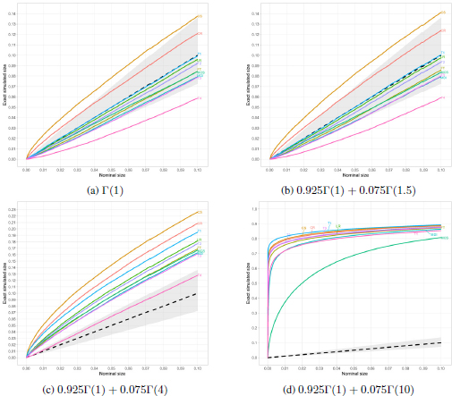
Figure 18.4. Exact simulated sizes against nominal sizes for the four cases of contamination. The gray area depicts the range of exact simulated sizes in which Dale’s criterion is satisfied. For a color version of this figure, see www.iste.co.uk/zafeiris/data1.zip
Results are presented in Figure 18.5, from where we can observe that under the adjustment the test statistics have similar behavior in terms of power for both cases of no contamination and contamination from the Γ(1), with the performance being downsized in the latter case. Note also that results under the adjustment differ from those of the preceding analysis. In particular, we can see that even though from Figure 18.3 we derived the conclusion that the best results arise for small values of α1 and large values of α2 in the no contamination case, T1 has the worst performance among all the BHHJ tests under the adjustment in size. Similar conclusions can be derived for the classical tests. For example, CS and CR have the worst performance among the classical tests under the adjustment, although in Table 18.2, results indicate the opposite. This behavior is explained by the fact that the power of the test is highly affected from its liberality or not, making the adjustment in size mandatory before proceeding to the comparison.
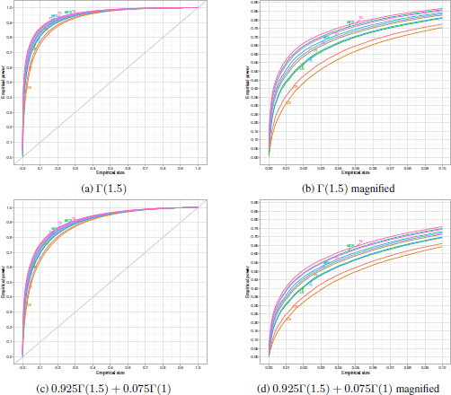
Figure 18.5. Left: empirical ROC curves for the no contamination and contamination from Γ(1) cases. Right: the same curves magnified over a relevant range of empirical sizes. For a color version of this figure, see www.iste.co.uk/zafeiris/data1.zip
In addition, taking into account the results of Figure 18.5, we focus our interest on the following four tests, two from each family, T 4, MCS, T 3 and MDI which appear to have the best performance in terms of power. Note that, even though MDI and T 3 closely follow each other in terms of size, T 3 appears to perform better in terms of power. Additionally, we can see that the performance of T 3 in terms of power closely follows the performance of MCS and especially when the alternative distribution is contaminated from the null. Although T 4 appears to have the best performance among all competing tests in terms of power, we should only consider it when the null distribution is contaminated from a distribution which is neither far nor close to the null since in every other case the exact simulated size fails to satisfy Dale’s criterion.
In conclusion, based on the analysis conducted with regard to the two families of estimators and test statistics, namely the BHHJ and the Cressie–Read families, we can state the following remarks. For estimation purposes, under contamination, the best estimators arise for large values of the index α2 and small negative values of the parameter λ, while the opposite is true when there is no contamination. In relation to testing procedures, when the null distribution is not contaminated or is contaminated from a distribution that is close to it, the best test statistics from the BHHJ family arise for values of the indices α1 and α2 close to 0.50, say between 0.40 and 0.60, while the most prominent members of the Cressie–Read family arise for values of λ ∈ [−2, −1]. In the case where the contaminant distribution lies neither too close nor too far from the null, only test statistics that are members of the BHHJ family with large values of α1 near 0.90 and moderate values of α2 near 0.30 are appropriate choices.
18.5. References
Ali, S.M. and Silvey, S.D. (1966). A general class of coefficients of divergence of one distribution from another. Journal of the Royal Statistical Society Series B, 28, 131–142.
Arndt, C. (2001). Information Measures. Springer, Berlin, Heidelberg.
Basu, A., Basu, S., Chaudhuri, G. (1997). Robust minimum divergence procedures for count data models. Sankhyā: The Indian Journal of Statistics Series B (1960–2002), 59(1), 11–27.
Basu, A., Harris, I.R., Hjort, N.L., Jones, M.C. (1998). Robust and efficient estimation by minimising a density power divergence. Biometrika, 85, 549–559.
Basu, S., Basu, A., Jones, M.C. (2006). Robust and efficient parametric estimation for censored survival data. Annals of the Institute of Statistical Mathematics, 58, 341–355.
Basu, A., Shioya, H., Park, C. (2011). Statistical Inference: The Minimum Distance Approach. Chapman & Hall/CRC Press, Boca Raton, FL.
Batsidis, A., Martin, N., Pardo Llorente, L., Zografos, K. (2016). ϕ-divergence based procedure for parametric change-point problems. Methodology and Computing in Applied Probability, 18(1), 21–35.
Cavanaugh, J.E. (2004). Criteria for linear model selection based on Kullback’s symmetric divergence. Australian & New Zealand Journal of Statistics, 46, 257–274.
Cover, T.M. and Thomas, J.A. (2006). Elements of Information Theory. John Wiley and Sons, New York.
Cressie, N. and Read, T.R.C. (1984). Multinomial goodness-of-fit tests. Journal of the Royal Statistical Society, 5, 440–454.
Csiszar, I. (1963). Eine Informationstheoretische Ungleichung und ihre Anwendung auf den Bewis der Ergodizitat on Markhoffschen Ketten. Publications of the Mathematical Institute of the Hungarian Academy of Sciences, 8, 84–108.
D’Agostino, R.B. and Stephens, M.A. (1986). Goodness-of-Fit Techniques. Marcel Dekker, New York.
Dale, J.R. (1986). Asymptotic normality of goodness-of-fit statistics for sparse product multinomials. Journal of the Royal Statistical Society. Series B (Methodological), 48(1), 48–59.
Ferentinos, K. and Papaioannou, T. (1979). Loss of information due to groupings. Transactions of the Eighth Prague Conference on Information Theory, Statistical Decision Functions, Random Processes, vol. C, 87–94, Reidel, Dordrecht-Boston, MA.
Ferentinos, K. and Papaioannou, T. (1983). Convexity of measures of information and loss of information due to grouping of observations. Journal of Combinatorics, Information & System Sciences, 8(4), 286–294.
Fisher, R.A. (1924). The conditions under which χ2 measures the discrepancy between observation and hypothesis. Journal of the Royal Statistical Society, 87, 442–450.
Ghosh, A., Maji, A., Basu, A. (2013). Robust inference based on divergence. In Applied Reliability Engineering and Risk Analysis: Probabilistic Models and Statistical Inference, Frenkel, I., Karagrigoriou, A., Lisnianski, A., Kleiner, A. (eds). John Wiley and Sons, New York.
Gokhale, D.V. and Kullback, S. (1978). The Information in Contingency Tables, vol. 23. Marcel Dekker, New York.
Kagan, A.M. (1963). On the theory of Fisher’s amount of information. Soviet Mathematics – Doklady, 4, 991–993.
Kateri, M. and Papaioannou, T. (1997). Asymmetry models for contingency tables. Journal of the American Statistical Association, 92(439), 1124–1131.
Kateri, M. and Papaioannou, T. (2007). Measures of symmetry-asymmetry for square contingency tables. TR07-3, University of Piraeus [Online]. Available at: https://www.researchgate.net/profile/Takis-Papaioannou-2/publication/255586795_Measures_of_Symmetry-Asymmetry_for_Square_%20Contingency_Tables/links/543147840cf27e39fa9eb943/Measures-of-Symmetry-Asymmetry-for-Square-Contingency-Tables.pdf.
Kateri, M., Papaioannou, T., Ahmad, R. (1996). New association models for the analysis of sets of two-way contingency tables. Statistica Applicata, 8, 537–551.
Kullback, S. (1985). Minimum discrimination information (MDI) estimation. In Encyclopedia of Statistical Sciences, Volume 5, Kotz, S. and Johnson, N.L. (eds). John Wiley and Sons, New York.
Kullback, S. and Leibler, R. (1951). On information and sufficiency. Annals of Mathematical Statistics, 22, 79–86.
Liese, F. and Vajda, I. (1987). Convex Statistical Distances. Teubner, Leipzig.
Lin, N. and He, X. (2006). Robust and efficient estimation under data grouping. Biometrika, 93(1), 99–112.
Lloyd, C.J. (2005). Estimating test power adjusted for size. Journal of Statistical Computation and Simulation, 75(11), 921–933.
Mathai, A. and Rathie, P.N. (1975). Basic Concepts in Information Theory. John Wiley and Sons, New York.
Mattheou, K. and Karagrigoriou, A. (2010). A new family of divergence measures for tests of fit. Australian and New Zealand Journal of Statistics, 52, 187–200.
Mattheou, K., Lee, S., Karagrigoriou, A. (2009). A model selection criterion based on the BHHJ measure of divergence. Journal of Statistical Planning and Inference, 139, 128–135.
Matusita, K. (1967). On the notion of affinity of several distributions and some of its applications. Annals of the Institute of Statistical Mathematics, 19, 181–192.
Menéndez, M.L., Morales, D., Pardo, L., Vajda, I. (2001). Approximations to powers of ϕ-disparity goodness-of-fit. Communications in Statistics – Theory and Methods, 30, 105–134.
Meselidis, C. and Karagrigoriou, A. (2020). Statistical inference for multinomial populations based on a double index family of test statistics. Journal of Statistical Computation and Simulation, 90(10), 1773–1792.
Nadarajah, S. and Zografos, K. (2003). Formulas for Renyi information and related measures for univariate distributions. Information Sciences, 155, 118–119.
Neyman, J. (1949). Contribution to the theory of χ2 test. In Proceedings of the 1st Symposium on Mathematical Statistics and Probability, University of Berkeley, 239–273.
Papaioannou, T. (1985). Measures of information. In Encyclopedia of Statistical Sciences, Vol. 5, Kotz, J. (ed.). Wiley, Hoboken, NJ.
Papaioannou, T., Ferentinos, K., Menéndez, M.L., Salicrú, M. (1994). Discretization of (h,ϕ)-divergences. Information Sciences, 77(3–4), 351–358.
Papaioannou, T., Ferentinos, K., Tsairidis, C. (2007). Some information theoretic ideas useful in statistical inference. Methodology and Computing in Applied Probability, 9(2), 307–323.
Pardo, L. (2006). Statistical Inference Based on Divergence Measures. Chapman & Hall/CRC, Boca Raton, FL.
Pardo, J.A. (2010). An approach to multiway contingency tables based on ϕ-divergence test statistics. Journal of Multivariate Analysis, 101, 2305–2319.
Patra, S., Maji, A., Basu, A., Pardo, L. (2013). The power divergence and the density power divergence families: The mathematical connection. Sankhya B, 75(1), 16–28.
Renyi, A. (1961). On measures of entropy and information. Proceedings of the Fourth Berkeley Symposium on Mathematical Statistics and Probability, 1, 547–561.
Sachlas, A. and Papaioannou, T. (2014). Residual and past entropy in actuarial science and survival models. Methodology and Computing in Applied Probability, 16(1), 79–99.
Shannon, C.E. (1948). A mathematical theory of communication. Bell Systems Technical Journal, 27(3), 379–423.
Toma, A. (2009). Optimal robust M-estimators using divergences. Statistics and Probability Letters, 79, 1–5.
Toma, A. and Broniatowski, M. (2011). Dual divergence estimators and tests: Robustness results. Journal of Multivariate Analysis, 102(1), 20–36.
Tsairidis, C., Ferentinos, K., Papaioannou, T. (1996). Information and random censoring. Information Science, 92(1–4), 159–174.
Tsairidis, C., Zografos, K., Ferentinos, K., Papaioannou, T. (2001). Information in quantal response data and random censoring. Annals of the Institute of Statistical Mathematics, 53(3), 528–542.
Victoria-Feser, M. and Ronchetti, E. (1997). Robust estimation for grouped data. Journal of the American Statistical Association, 92(437), 333–340.
Vonta, F. and Karagrigoriou, A. (2010). Generalized measures of divergence in survival analysis and reliability. Journal of Applied Probability, 47(1), 216–234.
Zografos, K. and Nadarajah, S. (2005). Survival exponential entropies. IEEE Transactions on Information Theory, 51, 1239–1246.
Zografos, K., Ferentinos, K., Papaioannou, T. (1986). Discrete approximations to the Csiszár, Rényi, and Fisher measures of information. Canadian Journal of Statistics, 14(4), 355–366.
Zografos, K., Ferentinos, K., Papaioannou, T. (1990). Divergence statistics: Sampling properties and multinomial goodness of fit and divergence tests. Communications in Statistics-Theory and Methods, 19(5), 1785–1802.
Chapter written by Christos MESELIDIS, Alex KARAGRIGORIOU and Takis PAPAIOANNOU.