
19
Geographically Weighted Regression for Official Land Prices and their Temporal Variation in Tokyo
This study models Tokyo official land price data using geographically weighted regression (GWR) and multi-scale GWR (MGWR) models. The GWR model spatially explores the varying relationships between land prices and the exploratory variables. Based on the estimated model parameters, the influence of land individuality increases as the estimated bandwidth parameters in the GWR model decrease. These facts are also confirmed by the local regression coefficients of the access index, the distance to the nearest station and residential area dummy variables. The differences between local coefficients for some convenience indicators, including access time to central Tokyo and walking distances to nearest stations, tend to increase between the west and central areas of Tokyo.
19.1. Introduction
In the “price announcement of public land”, published annually in March, the Ministry of Land, Infrastructure, Transport and Tourism (MLIT) of Japan announces the prices of standard land on January 1 based on the Land Price Announcement Law. This announcement not only provides an appropriate index of land prices for general land transactions, but also plays the role of institutional infrastructure in the socio-economic context, being applied to national land use plans, including land acquisition and planning for public work projects. The price announcement of public land is thus not only the standard for evaluating inheritance and fixed property taxes, but is also an important index that reflects the actual state of land prices. While strict evaluation procedures are set for normal land prices, the price announcements of public land are stationary observations, and since survey points can change frequently, it is difficult to monitor land prices at the same time points over a long period of time. Thus, in this study, we analyze the changes in the price announcements for public land using the geographically weighted regression (GWR) and the multi-scale GWR (MGWR) models for a total of 38,914 residential use land areas in Tokyo based on price announcements for public land from 1997 to 2018.
The GWR model was proposed by Brunsdon et al. (1996) and Fotheringham et al. (1998) as a spatial statistical model considering spatial heterogeneity. In other words, the GWR model is a local regression model that captures spatial heterogeneity or non-stationarity by estimating spatially varying regression coefficients. One of the disadvantages of the GWR model is that the multicollinearity between explanatory variables occurs when using a common bandwidth for spatial kernels for all explanatory variables, which yields similar or unstable regression coefficients for the target area. Hence, various models that extend the GWR model have been proposed and applied in the literature. For instance, the mixed GWR model is a mixed model of linear regression and GWR, which attempts to explain both the global variables common to all observations and the local variations in the characteristics of each site (Lee et al. 2009). In this study, we overcome the shortcomings of the GWR model by using the MGWR model, which estimates the local regression coefficients using variable-specific bandwidth for spatial kernels (Lu et al. 2017)1.
Various global GWR applications also exist in the literature. For example, Cho et al. (2006) estimated the GWR model using housing data from Knox County, Tennessee, showing that the proximity of water areas and parks to housing is reflected in the price. Helbich et al. (2014) estimated a mixed GWR model that distinguishes between local and global explanatory variables based on Australian residential data. Using sample size-based distance measures for spatial kernels, Lu et al. (2015) argued that the fitting performance is better than that for the usual distance-based kernels, and constructed a parameter-specific distance metrics-GWR (PSDM-GWR) model using both distinct bandwidth and metric functions of each explanatory variable. Additionally, they proposed back-fitting algorithms to fit the generalized linear model with the parameter estimation of PSDM-GWR models. Lu et al. (2017) estimated GWR and MGWR models using housing transaction prices in London in 2001, and showed that the MGWR model is superior in terms of fitting and prediction accuracy. Recently, several studies extended the GWR and MGWR models to the space–time dimensions, including that of Huang et al. (2010). LeSage and Pace (2009) derived estimates focusing on the results of spatiotemporal long-term equilibrium with regard to the use of cross-sectional data and focusing on the dynamics embodied by time-dependent parameters with regard to the use of spatiotemporal data.
In this study, we assume independence between the different time points and estimate secular changes under the GWR and MGWR models. This study thus clarifies the interannual variability of geographical and environmental factors for land prices by applying the GWR and MGWR models. Our findings are as follows. For over 20 years, the individual factors of land prices increase, as demonstrated by the increase in the local regression coefficients in Tokyo. Additionally, due to the secular changes in environmental factors that indicate convenience, the land price differences between the central and southern parts of the 23 wards, including the surrounding and other areas, increase. In particular, in the western part of Tokyo, the estimates of the MGWR model show that the land price differences in the eastern part increase towards the west. Moreover, the influence of higher land prices was stronger in the southern part of Kitatama (Northern Tama Area) than in the northeastern part of the 23 wards. There are also regional differences in land preferences. From the central to the northern areas of the 23 wards and from the western area of Kitatama to the eastern area of Nishitama (Western Tama Area), low-rise residential areas that have an emphasis on the living environment are preferred. Conversely, in the Minamitama (Southern Tama) area, residential areas and semi-residential areas that have an emphasis on convenience and commerciality are preferred. Each influence became stronger as time progressed. Furthermore, the above-mentioned effects significantly changed before the 2008 financial crisis and remained stable after the crisis.
The rest of this chapter is structured as follows. In section 19.2, we explain the GWR model, which is a spatial econometric model that considers both spatial dependence and spatial heterogeneity, and its extension, the MGWR model. section 19.3.1 presents the data used to obtain the land price function. In section 19.3.2, we estimate the non-spatial model by OLS, GWR and MGWR using published land prices. Additionally, we consider secular changes by visualizing the spatial prediction distribution of the parameters. Finally, section 19.4 summarizes and discusses the results.
19.2. Models and methodology
We denote yt(s) by the logarithmic public land price vector of site s ∈ D in region D at time t. Then, the global or non-spatial model can be expressed as follows:
where Xt(s) is the matrix of the explanatory variables described in the previous section, βt is the vector of the regression coefficient, including the constant term, and εt(s) is the error term, which is assumed to be independent at time t and for site s. x′ denotes the transpose of a matrix or vector x. The regression coefficients of the non-spatial models are common for all sites.
The GWR uses location-wise estimates to model spatially varying relationships. Let yt(si) be the logarithmically transformed official land price of each site si with n observation sites (si, i = 1,..., n) at time t. Further, let the k-dimensional vector of the explanatory variable be Xt(si)= [1, x1,t(si), ··· , xk−1,t(si)]′. We denote the vector of local regression coefficients by βt,i(k × 1) and the error term by εt(si). Then, the GWR model can be expressed as:
Under the GWR, to estimate βt,i = [β0,t,i, β1,t,i, ··· , βk−1,t,i]′, we use the generalized least-squares (GLS) method using the following weight matrix:
Here, matrix Vt,i is a diagonal matrix and its j-th component vt,i,j is the weight given to site j:
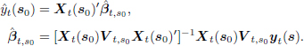
The estimator of the local regression coefficient at site i and time t is given by:
In the GWR model, it is important to define weight matrix Vt,i. To this end, we use a Gaussian distance-decay function:
where di,j is the Euclidean distance between i and j. δt is the bandwidth of a common spatial kernel at time t. Bandwidth δt is determined by minimizing the cross-validation (CV) error of the following equation:
where ![]() is the predicted value for the neighbor of site i, without using site i. If the spatial distribution of the observed points is not constant, an adaptive kernel that adjusts the bandwidth according to the number of samples, not the distance, may be used; see, for example, Lu et al. (2015).
is the predicted value for the neighbor of site i, without using site i. If the spatial distribution of the observed points is not constant, an adaptive kernel that adjusts the bandwidth according to the number of samples, not the distance, may be used; see, for example, Lu et al. (2015).
Let the explanatory variable for site s0 be Xt(s0). Then, the predicted value of the log official land price becomes:
See, for example, Leung et al. (2000) and Harris et al. (2011). The corresponding variance of the predictor becomes:

where ![]() is the variance of error term ε(s0) for site s0.
is the variance of error term ε(s0) for site s0.
Brunsdon et al. (1999) pointed out that, for the GWR and mixed GWR models, the bandwidths of the common spatial kernels are sometimes restrictive and the resulting GWR estimates tend to be inflexible. Additionally, Wheeler and Tiefelsdorf (2005) explained that, under the GWR model, there exists instability that creates multicollinearity due to the similarities of local explanatory variables. Hence, Yang (2014) proposed the MGWR model, which applies a distinct bandwidth for each explanatory variable for the spatial kernels. The MGWR model can provide more location-specific regression surfaces, which makes it possible to avoid multicollinearity between variables. In this study, we use the following extended algorithm, as proposed by Lu et al. (2017).
Step 0: Data formatting: we denote the data matrix and log land price by yj,t and Xt, respectively, for time t(1 ≤ t ≤ T ) and site i(1 ≤ i ≤ p). Let ![]() be the initial weight matrix for t, i, and the k-th regression coefficients in the GWR model. The initial kernel bandwidth is set to
be the initial weight matrix for t, i, and the k-th regression coefficients in the GWR model. The initial kernel bandwidth is set to ![]() . The required precision is denoted by τ > 0, and the maximum number of iterations is set as ℕ.
. The required precision is denoted by τ > 0, and the maximum number of iterations is set as ℕ.
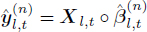
Step 1: Initialization: initial estimates ![]() are obtained by the GWR model. Then, we calculate
are obtained by the GWR model. Then, we calculate ![]() . Here, Xh−1,t denotes the h-th row of matrix Xt and ◦ is the Hadamard product. We obtain the residual sum of squares,
. Here, Xh−1,t denotes the h-th row of matrix Xt and ◦ is the Hadamard product. We obtain the residual sum of squares, ![]() .
.
Step 2: update the (n)-th estimates using the estimates of the (n − 1)-th iteration as follows. Here, we re-define the explanatory variable as Xl,t(0 ≤ l ≤ m).
- 1) Calculate
 , where
  denotes the sum of numbers other than l and
- 2) We calculate bandwidth
 using criteria such as the CV scoring method and obtain weight matrix
  .
. Finally, we calculate
 by using
  and Xl, t.
 - 3) We update
 .
.
Step 3: Using ![]() , we calculate
, we calculate ![]() and RSS(n) and obtain the rate of change CVR(n):
and RSS(n) and obtain the rate of change CVR(n):
If CVR(n) < τ or ![]() , the calculation ends. Otherwise, n = n + 1 and the process is repeated.
, the calculation ends. Otherwise, n = n + 1 and the process is repeated.
19.3. Data analysis
19.3.1. Data
The public announcement of land prices in 2018 was conducted for 47 prefectures nationwide in Japan, targeting 20,572 areas for urbanization, 1,394 urbanization control areas, 4,015 other urban planning areas and 19 publicly announced areas outside the urban planning area, for a total of 26,000 standard land areas. In Tokyo, there were 2,602 sites and 1,540 residential zones, excluding islands. In this study, we use the public announcement of land price data for residential zoning in Tokyo as of January 1, 1997 to 2018. A total of 38,914 data points exist during the 22-year analysis period. The number of sites subject to the public announcement of land prices for residential zoning changed annually as needed, which varies from 1,200 to 2,000.
We estimate each model using the official land price as the objective variable. As explanatory variables, we selected the following seven variables: (1) access index of the target site (minutes), (2) distance to the main nearest station (m), (3) front road width (m), (4) land area of the target site (m2), (5) low-rise residential area dummy, (6) residential area dummy, and (7) gas equipment dummy. All variables except for the dummy ones are transformed into logarithmic values.
Figure 19.1 shows a boxplot of the transitions in official land prices for 22 analyzed years. There are outliers above the boxplot due to the presence of very high land prices. The average official land price at the analysis sites was 393,000 yen/m2 in 2018, and the median value was 310,000 yen/m2. Regarding the time-series transitions, land prices had been declining since 1997 until the early 2000s and then rose until 2008, after which they showed a downward trend once more due to the effects of the 2008 financial crisis. In recent years, the upward trend of high official land price sites has been remarkable. Figure 19.2 shows the distribution of official land prices in the residential areas of Tokyo in 2018. The highest official land price was 4,010,000 yen/m2 and the lowest was 45,000 yen/m2. The official land prices are generally high near the central area of the 23 wards, which is also the center of the city, but they are not always high within the other 23 wards, except for the Adachi, Katsushika and Edogawa wards in the northeastern part of Tokyo and Musashino City and Mitaka City, which are adjacent to the 23 wards to the west. Additionally, the locations and numbers of public notice points are highly biased by region.

Figure 19.1. Boxplots of official land prices in Tokyo from 1997 to 2018

Figure 19.2. Spatial distributions of Tokyo official land prices in 2018
19.3.2. Results
Here, we perform the parameter estimation using the models presented in section 19.2, namely the non-spatial model, GWR model and MGWR model. A non-spatial model is a global regression model whose coefficients are common for all sites and are estimated by OLS. For GWR and MGWR models, the local regression parameters that show the spatial patterns and heterogeneity are estimated.
Table 19.1. Regression coefficients for the non-spatial and GWR models for 2018
| Non-spatial model GWR model ( | |||||||
| SE | Min | Q1 | Median | Q3 | Max | ||
| Intercept | 17.3990 | 0.1181 | 2.3637 | 14.1987 | 15.4629 | 18.1178 | 38.9184 |
| Access index | -1.0633 | 0.0182 | -5.4377 | -1.1618 | -0.5631 | -0.2583 | 1.5504 |
| Distance to station | -0.2770 | 0.0112 | -0.4836 | -0.2392 | -0.1772 | -0.1208 | 0.1633 |
| Front road width | 0.1430 | 0.0218 | -0.2991 | 0.0368 | 0.0916 | 0.1664 | 0.7921 |
| Land area | 0.1378 | 0.0150 | -0.7251 | -0.0106 | 0.0488 | 0.1125 | 1.3120 |
| Low-rise residential | 0.0098 | 0.0181 | -0.6611 | -0.1087 | -0.0275 | 0.0456 | 0.5553 |
| Residential | -0.0099 | 0.0217 | -0.6033 | -0.0683 | 0.0153 | 0.0993 | 0.4892 |
| Gas equipment | -0.2836 | 0.0273 | -2.2197 | -0.7126 | -0.3128 | -0.1007 | 1.1098 |
Table 19.1 shows a comparison of the regression coefficients for the non-spatial and GWR models. Under the non-spatial model, the low-rise residential area and residential area dummies are insignificant at the 5% significance level. The local regression coefficient on the GWR model is estimated for each site, and there is a range in the distribution of the regression coefficients. If we compare the median values of the regression coefficients estimated by the GWR model, then the absolute value of the estimates, which was significant under the non-spatial model, becomes smaller. Table 19.2 shows a comparison with the MGWR model. If we compare the regression coefficients on the median values, the estimates for the GWR and MGWR models take similar values, but smaller absolute values under the non-spatial model. The range of each regression coefficient, which was large under the GWR model, is smaller under the MGWR model, probably because of the common bandwidth for spatial kernels for all explanatory variables. Specifically, this bandwidth might be too large or too small for each variable in the GWR model and was estimated adequately under a variable-specific bandwidth for spatial kernels in the MGWR model.
Figure 19.3 shows the time-series transition of the estimated regression coefficients under the GWR model. The Gaussian distance-decay function is adopted, and the common bandwidth for the spatial kernels is determined by the CV scoring method, according to equation [19.1]. Except for the intercept, the range of the regression coefficients on the access index and gas equipment dummy is larger than for the other regression coefficients. Additionally, outliers are present for all regression coefficients. The regression coefficients on the access index, nearest station distance and the gas equipment dummy took on a negative trend in recent years, similar to the non-spatial model. This fact indicates that, if both explanatory variables are at the same level, the effect of reducing land prices becomes stronger over time. No visual trend is observed for the coefficients on the other explanatory variables.
Table 19.2. Regression coefficients for the GWR and MGWR models for 2018
| GWR model | MGWR model | |||||||
| Mean | SD | Min | Q1 | Median | Q3 | Max | ||
| Intercept | 16.4557 | 2.6373 | 12.9792 | 13.8973 | 15.1192 | 19.2707 | 21.2709 | 0.58 |
| Access index | -0.7830 0.6063 | -1.6806 | -1.4486 | -0.4205 | -0.1955 | -0.1586 | 2.52 | |
| Distance to station | -0.1695 0.0443 | -0.2592 | -0.1972 | -0.1720 | -0.1112 | -0.0664 | 3.76 | |
| Front road width | 0.0972 0.0143 | 0.0749 | 0.0833 | 0.0987 | 0.1102 | 0.1172 | 14.41 | |
| Land area | 0.0414 0.0758 | -0.1907 | -0.0063 | 0.0423 | 0.0891 | 0.2231 | 1.90 | |
| Low-rise residential | -0.0065 0.0902 | -0.3621 | -0.0373 | 0.0047 | 0.0463 | 0.1654 | 2.37 | |
| Residential | 0.0244 0.0302 | -0.0277 | -0.0027 | 0.0165 | 0.0478 | 0.0958 | 6.81 | |
| Gas equipment | -0.4706 0.3869 | -1.1953 | -0.8197 | -0.4709 | -0.0785 | 0.0500 | 3.38 | |
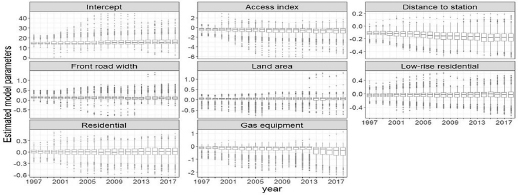
Figure 19.3. Boxplots of the transition for the estimated GWR model parameters
Figure 19.4 shows the time-series transition of the estimated regression coefficients under the MGWR model using boxplots. We use the algorithm of Lu et al. (2017) for parameter estimation. The bandwidth for the variable-specific spatial kernels is determined by converging the CVR in equation [19.2]. Compared to the GWR model, the range of the regression coefficients is smaller and the vertical length of the boxplot becomes longer with fewer outliers. In addition to the access index and nearest station distance, a negative trend can be confirmed for front road width and the gas equipment dummy, and a positive one for the low-rise residential area dummy. The range of the boxplots for the access index, nearest station distance, low-rise residential area dummy and residential area dummy becomes larger over time, which indicates that the individual factor of land for the explanatory variable becomes stronger with respect to land price. Additionally, the increase in the range of the constant terms means that the individual factors of land for the explanatory variables not used in this analysis are likely increasing2.

Figure 19.4. Boxplots of the transitions for the estimated parameters under the MGWR model
Table 19.3. Fitting performances of the models for 2018
| Non-spatial model | GWR model | MGWR model | |
| Kernel bandwidth (km) | — | 1.41 | 0.58 – 14.41 |
| Adjusted R2 | 0.8492 | 0.9746 | 0.9821 |
| AICc | 365.18 | -1632.58 | -2024.02 |
| MSE | 0.0734 | 0.0067 | 0.0040 |
| Prediction accuracy (%) | 21.9019 | 5.9864 | 4.5662 |
| Moran’s I of residuals | 0.5004 (pvalue 0.0000) | 0.0063 (pvalue 0.1585) | -0.0336 (pvalue 1.0000) |
Table 19.3 summarizes the fitting performances of the non-spatial, GWR and MGWR models by the land price function in 2018. The MSE indicates the mean-squared error, and the prediction accuracy is defined by the following equation [19.3]:
Regarding the goodness of fit, it is desirable that the AICc and prediction accuracy (%) are small and the adjusted R2 is close to 1. As for the spatial correlation of residuals, it is desirable that Moran’s I is close to 0 because the spatial correlation cannot be confirmed for the error term if the spatial regression model is fitted properly. From this table, the MGWR model outperforms the non-spatial and GWR models in 2018.
Figure 19.5 shows the time-series transition of the fitting performance for each model. The MGWR model has the best fit of the three models every year. Since the adjusted R2 of the non-spatial model changes to around 0.84, the non-spatial model can explain a large proportion of the official land price, but residual Moran’s I is around 0.50. If there is a spatial correlation, the adjusted R2 is overestimated. The fit of the GWR and MGWR model is significantly better than that of the non-spatial model, as the adjusted R2 of the GWR model is around 0.97 and the AICc ranges from −4,000 to −1,500. Since the transition of residual Moran’s I is around 0.03, no significant spatial correlation is observed. In the MGWR model, the adjusted R2 is around 0.98 and the AICc is from −5,000 to −2,000, which is even better than for the GWR model and the MSE and prediction accuracy are also improved. The change in residual Moran’s I ranges from −0.04 to −0.03, and no significant spatial correlation is observed even at the 1% level. Additionally, the MSE and prediction accuracy of the MGWR model and residual Moran’s I are stable.

Figure 19.5. Transition of the performance measure fit
Figure 19.6 shows the time-series transition of the bandwidth for the variable-specific spatial kernels under the MGWR model. The “GWR” label in the top-right panel indicates the common bandwidth for spatial kernels under the GWR model. Under this model, the kernel bandwidth changed from 1.4 km to 1.9 km. After the burst of the bubble economy, the range of official land prices narrowed during their downward trend, and has remained stable since then. Under the MGWR model, the trend in the kernel bandwidth for each explanatory variable was confirmed, regardless of the trend of official land prices. The kernel bandwidth of the constant term is smaller than that for the other explanatory variables due to the increase in the individual factors of land over time that cannot be explained by the explanatory variables included in this study. Moreover, the access index, nearest station distance, front road width, residential area dummy, gas equipment dummy kernel and the bandwidth are allowed to jump from 2013 to 2016. The cause is thought to be a large change in the number of publicly announced points. The fact that the kernel bandwidth of the front road width is larger than those of the other explanatory variables and an upward trend can be seen in recent years indicates that it may become a global explanatory variable. We would like to consider these cases in future research.
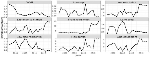
Figure 19.6. Transition of bandwidth for variable-specific kernels under the MGWR model and the common bandwidth for the GWR model
19.4. Conclusion
This study estimated a land price model using 38,914 sites over 22 years of residential area of Tokyo. Three models were compared based on their fitting performances, namely the non-spatial, GWR and MGWR models. We found that the MGWR model with variable-specific bandwidth for spatial kernels has a better fit than the non-spatial and GWR models in terms of the adjusted R2, AICc, MSE, prediction accuracy and spatial correlation of residuals. The results of the MGWR model and its visualization confirmed that the individuality of the land, which is a factor of land price formation, is gradually strengthened by the increase in the range of each local regression coefficient. The effects of the access index, nearest station distance and low-rise residential area dummy are remarkable. Additionally, from the increase in the range of constant terms, the individuality of the land other than the explanatory variables used in this study strengthened.
A future research project is to build an MGWR model that includes global explanatory variables and extend it to the space–time dimension. The mixed GWR model estimates the parameters of the regression model by distinguishing between global and local explanatory variables, but the local explanatory variables use a common bandwidth for spatial kernels. The GWR model considers spatial effects such as spatial autocorrelation and spatial heterogeneity, while the MGWR model is an advanced version of it. However, because of the nature of the explanatory variables, they are not always spatially affected. We will consider constructing a mixed MGWR model that quantitatively measures the characteristics of the explanatory variables and enhances the consistency of the model in future studies. Additionally, Huang et al. (2010) and Fotheringham et al. (2015) proposed a geographically and temporally weighted regression model (GTWR) with weights for both the space and time dimensions for Calgary, Canada and London, respectively, and reported that the GTWR model improved the forecasting accuracy. Further, Wu et al. (2019) proposed an MGTWR model, which is a multi-scale version of the GTWR and estimated the land price model in Shenzhen, Guangdong Province, China. Analyzing these models is a future research topic. Moreover, it is necessary to consider the explanatory variables of the land price function and its form. In particular, as per Chay and Greenstone (2005) and Heckman et al. (2010), it is necessary to construct a nonlinear model that considers the size and age of households and the spatial heterogeneity of their characteristics in estimating the land price function.
19.5. Acknowledgments
This research was supported in part by JSPS KAKENHI Grant Number 18K01706 and Nanzan University Pache Research Subsidy I-A-2 for the 2021 academic year.
19.6. References
Brunsdon, C., Fotheringham, A.S., Charlton, M.E. (1996). Geographically weighted regression: A method for exploring spatial nonstationarity. Geographical Analysis, 28(4), 281–298.
Brunsdon, C., Fotheringham, A.S., Charlton, M.E. (1999). Some notes on parametric significance tests for geographically weighted regression. Journal of Regional Science, 39(3), 497–524.
Chay, K.Y. and Greenstone, M. (2005). Does air quality matter? Evidence from the housing market. Journal of Political Economy, 113(2), 376–424.
Cho, S.H., Bowker, J.M., Park, W.M. (2006). Measuring the contribution of water and green space amenities to housing values: An application and comparison of spatially weighted hedonic models. Journal of Agricultural and Resource Economics, 31(3), 485–507.
Fotheringham, A.S., Charlton, M.E., Brunsdon, C. (1998). Geographically weighted regression: A natural evolution of the expansion method for spatial data analysis. Environment and Planning A, 30(11), 1905–1927.
Fotheringham, A.S., Crespo, R., Yao, J. (2015). Geographical and temporal weighted regression (GTWR). Geographical Analysis, 47(4), 431–452.
Harris, P., Brunsdon, C., Fotheringham, A.S. (2011). Links, comparisons and extensions of the geographically weighted regression model when used as a spatial predictor. Stochastic Environmental Research and Risk Assessment, 25(2), 123–138.
Heckman, J.J., Matzkin, R.L., Nesheim, L. (2010). Nonparametric identification and estimation of nonadditive hedonic models. Econometrica, 78(5), 1569–1591.
Helbich, M., Brunauer, W., Vaz, E., Nijkamp, P. (2014). Spatial heterogeneity in hedonic house price models: The case of Austria. Urban Studies, 51(2), 390–411.
Huang, B., Wu, B., Barry, M. (2010). Geographically and temporally weighted regression for modeling spatio-temporal variation in house prices. International Journal of Geographical Information Science, 24(3), 383–401.
Lee, S., Kang, D., Kim, M. (2009). Determinants of crime incidence in Korea: A mixed GWR approach. World Conference of the Spatial Econometrics Association, Barcelona.
LeSage, J.P. and Pace, R.K. (2009). Introduction to Spatial Econometrics. Chapman and Hall/CRC, Boca Raton, FL.
Leung, Y., Mei, C.L., Zhang, W.X. (2000). Statistical tests for spatial nonstationarity based on the geographically weighted regression model. Environment and Planning A, 32(1), 9–32.
Lu, B., Harris, P., Charlton, M., Brunsdon, C. (2015). Calibrating a geographically weighted regression model with parameter-specific distance metrics. Procedia Environmental Sciences, 26, 109–114.
Lu, B., Brunsdon, C., Charlton, M., Harris, P. (2017). Geographically weighted regression with parameter-specific distance metrics. International Journal of Geographical Information Science, 31(5), 982–998.
Wheeler, D.C. and Tiefelsdorf, M. (2005). Multicollinearity and correlation among local regression coefficients in geographically weighted regression. Journal of Geographical Systems, 7(2), 161–187.
Wu, C., Ren, F., Hu, W., Du, Q. (2019). Multiscale geographically and temporally weighted regression: Exploring the spatiotemporal determinants of housing prices. International Journal of Geographical Information Science, 33(3), 489–511.
Yang, W. (2014). An extension of geographically weighted regression with flexible bandwidth. PhD Thesis, St Andrews.
Chapter written by Yuta KANNO and Takayuki SHIOHAMA.
- 1 Both mixed GWR and multi-scale GWR are sometimes referred to as MGWR but, to avoid confusion, we refer to multi-scale GWR as MGWR.
- 2 The individual factors of land include areas of caution on hazard maps, the existence of crime, local sunshine and noise conditions, as well as the location of garbage collection sites.