
22
Using Parameters of Piecewise Approximation by Exponents for Epidemiological Time Series Data Analysis
Nowadays, detailed epidemiological data are available in the form of time series data (or as an array): N[k] – where N is the documented number of events registered at the equidistant time moments T(k) = To + k*delta (e.g. “Number of newly reported cases of Covid-19 in the last 24 hours” – published on a daily basis by WHO). Theoretically, those data can be adequately described by different dynamic models containing exponential growth and exponential decay elements. Practically, parameters of those models are not constants – they can change in time because of many factors like changing hygiene policies, changing social behavior and vaccination. Hence, it was decided to use a piecewise approach: short sequential fragments of time series data are approximated by a function containing some parameters. The above parameters are evaluated for the first time series data fragment. Then, the next data fragments are processed. As a result, new time series data (arrays) are created: evaluated sequences of parameters. Those new series can be considered and analyzed as functions of time. In the simplest example, the function to be used for every fragment is A + B*exp( alpha* t). The resulting values of A, B and alpha in that case are time series data – arrays: A[k], B[k] and alpha[k] known at the equidistant time moments T(k). By plotting those sequences, it can be seen if the simple growth or decay model is adequate. Significant jumps in values may point to an interesting event, for example the start of mass vaccination or the effect of a non-desirable social behavior on the specific date. In order to make calculations robust, some preliminary filtration and after-filtration can be used (e.g. by using moving average, moving median or other filters such as the Gaussian filter and Bessel filter). A number of practical examples were considered.
22.1. Introduction
The plurality of epidemiology models is known. The simplest (classical models) described epidemic data in terms of exponential growth and decay, see, for example, “A tutorial for students” by Okabe and Shudo (2020). More sophisticated mathematical models use a set of linear or nonlinear differential equations with a set of empirical parameters – from the classic SIR epidemic model (using compartments with labels S for Susceptible, I for Infectious and R for Recovered) created by Kermack and McKendrick (1927), to its different modifications listed in a constantly updated list in Wikipedia. The problem with those models is that they consider parameters as constants, which, in the best case, is only a theoretically reasonable assumption. In real life, parameters of the models are influenced by a number of non-epidemiological factors – for example, by executing (or not executing) some specific policy, by changing hygiene policies, by changing social behavior and by time of vaccination. In this chapter, the “local piecewise approach” will be used to analyze epidemiological time series data.
22.2. Deriving equations for moving exponent parameters
In real-life measurements, time series data are typically described as an array of digital values obtained from measurements provided at the equidistant time points. In electronics, for example, such an array is treated as a “signal”. A large number of DSP (digital signal processing) algorithms are known and widely used. Probably the simplest DSP algorithm is a “moving average” (rolling average and running average). Input data are described by an array Y[k] of a fixed size. Values of Y are known for the equidistant time marks T[k] =To + k*delta; index k is changed from “1” to “N”, where N is a number of measured values of Y. In some programming languages such as C and C++ (typically used in the implementation of the DSP algorithms), index “k” is started from 0, and maximal index is (N-1); however, in this chapter, starting index “1” will be used. For the simplest three-taps moving average, the resulting (processed) array is Z[k]. For an arbitrary index “k”, Z[k] is calculated as (Y[k-1]+Y[k]+Y[k+1])/3. It is clear that values of Z[1] and Z[N] cannot be calculated by using this formula. In some implementations above, values are set to 0 or to NaN. In some implementations, resulting array Z has a size (N-2). In the last case some time shift is created and, thus, this time shift must be taken into account. The resulting Z (if treated as a signal) represents the filtered signal Y. Practically, more sophisticated filters must be used to filter “noise”. The idea of this approach will be used here to describe signal Y as a sequence of time shifted piecewise exponents. In that case, the resulting “signals” will be parameters of “moving exponents”. In some approximations, algorithm data are approximated by an exponential function A*exp(-alpha*t), where A and “alpha” are the parameters to be found. Practically, to find values of “A” and “alpha” logarithms (and log graphs) are used. However, this approach works only if values of “A” and “alpha” are constants – at least for the time interval selected for measurements.
To analyze the situation when parameters of the function used for the approximation may change, the following approach (analogous to approach used in the “moving average”) will be used.
To derive equations in the symbolic form and to provide numerical calculations, and present results as graphs, MAPLE software was used. In the following description of the method selected, self-explanatory fragments of MATLAB code will be used.
The following function was used to approximate short fragments of original data:
Y := proc (t, A, B, alpha)
A+B*exp ( alpha *t):
end proc
It is known that if three values of some signal Y1, Y2 and Y3 are known for equidistant points of “t”, “t+delta” and “t+2*delta”, then parameters A, B and alpha can be found by solving the following equations:
Equ1 := A+B*exp(alpha*t) = Y1
Equ2 := A+B*exp(alpha*(t+delta)) = Y2
Equ3 := A+B*exp(alpha*(t+2*delta)) = Y3
After using MAPLE procedure “solve”
Solution 1 := solve({Equ1, Equ2, Equ3}, {A, B, alpha})
and after operating MAPLE simplifications, the following formulae for the parameters A, B and alpha were obtained:
A := (Y1*Y3-Y2^2) / (-2*Y2+Y3+Y1)
B := (Y2-Y3)*(Y1-Y2)*((Y2-Y3)/(Y1-Y2))^((-delta-t)/delta)/(-2*Y2+Y3+Y1)
alpha := ln ( (Y2-Y3) / (Y1-Y2) ) / delta
It can be seen that formulae for “alpha” and “A” are relatively simple for practical implementation. However, the equation for “B” is slightly problematic for the goals of this analysis because, obviously, the value of B depends on the value of “t”. This behavior can be compensated but to do this, some “starting” moment of “t” must be set. Hence, in this chapter, only values of A and alpha will be analyzed for the real data. It can be noted that while for the symbolic calculations the above formulae are adequate, for the numerical calculations some real-life numerical data combinations of values may become problematic. For example, if (-2Y2 +Y3+Y1) is equal to zero, then numerical calculations of A and B cannot be executed. For numerical calculation of “alpha”, the following “protected” procedure was used:
AlphaF := proc (Y1, Y2, Y3, delta)
local x, y; x := (Y2-Y3)/(Y1-Y2);
if x < = 0 then y := 0
else y := evalf( ln(x) / delta )
end if;
return y
end proc;
It must be noted that this protection added “impulse noise”. However, this noise can be effectively eliminated by using the median filter.
22.3. Validation of derived equations by using synthetic data
To validate the proposed approach, synthetic data were used. To make calculations, plotting and analysis simple, the size of the “TestData” array was set to the relatively small number of 64. Values of “TestData” were calculated as a combination of two exponents having different amplitudes and “alpha”. The first exponent “started” at the time “0”, whereas the second exponent started after a time delay equal to 32 time intervals “delta”. The following fragment of the code demonstrates how values of “TestData” were calculated:
for k to arraySize do
TestData[k]:= evalf(TestA1*(1-exp(k/TestK1))
+Heaviside(k-(1/2)
*arraySize)*TestA2*(1-exp((k-(1/2)*arraySize)/TestK2)))
end do
Parameters were set as: TestA1 = 300, TestK1 = -8. TestA2 = 500, TestK2 = -5.
Figure 22.1 presents the synthetic data in graphical form. The presented signal is typical in the field of digital electronic signals.
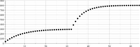
Figure 22.1. “TestData” created by calculations. Axes “Y”: values of “TestData”. Axes “X”: time ticks in the range {1..64}
From Figure 22.1, it can be seen that “the second exponent” started at moment 32. It can be seen that at this time, “the first exponent” (that started at moment “1”) practically became a constant.
The array “TestData” was processed by way of “moving average”, but instead or “average”, parameters “Alpha”, “A” and “B” were calculated for the different values of the index “k”. Parameter TestDataStep was set to “1” here.
for k from 2 to arraySize-1 do
Zalpha[k] := evalf(AlphaF(TestData[k-1], TestData[k], TestData[k+1], 1));
Za[k] := evalf(AoF(TestData[k-1], TestData[k], TestData[k+1], 1));
Zb[k] := evalf(BoF(TestData[k-1], TestData[k], TestData[k+1], 1, k))
end do
This procedure effectively creates new data series (arrays): “Zalpha[k]”, “Za[k]” and “Zb[k]”. Figure 22.2 presents the array “Zalpha” and Figure 22.3 represents the array “Za”.
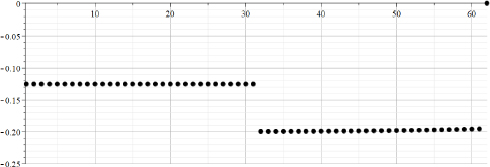
Figure 22.2. Calculated array “Zalpha” after median filtration. Axes “Y”: values of “Zalpha”. Axes “X”: counts in the range {1..64}
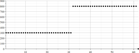
Figure 22.3. Calculated array “Za” after median filtration. Axes “Y”: values of “Za”. Axes “X”: counts in the range {1..64}
The values of Zalpha represent the calculated values of the parameter “alpha” for the different moment of time. From Figures 22.2 and 22.3, we can clearly see that in the left part, “the signal” can be described as an exponent having “alpha” = -0.125 = -1/8 and magnitude A = 300, whereas in the right part, “the signal” can be described as an exponent having “alpha”= -0.2 = -1/5, and magnitude A = 300+500 = 800.
It can be concluded that in this case, the description by a “moving exponent” is adequate, and that calculated values coincide with the values that were used for the calculations of “TestData”.
22.4. Using derived equations to analyze real-life Covid-19 data
Real-life Covid-19 data were downloaded as an Excel file from the site (Ritchie et al. 2021). This file contains data for a large number of countries. To demonstrate use of the developed approach, the data concerning Israel and Sweden were used.
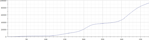
Figure 22.4. Total number of Covid-19 cases per million (Israel)
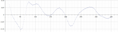
Figure 22.5. Values of “alpha” calculated by using data of Figure 22.4
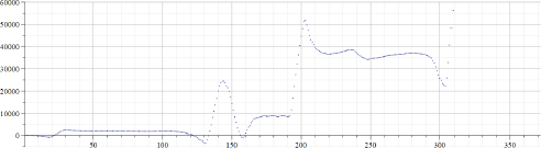
Figure 22.6. Values of “A” calculated by using data of Figure 22.4
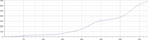
Figure 22.7. Total number of deaths per million (Israel)
Original data for the “total number of Covid-19 cases per million” in Israel published in the source (Ritchie et al. 2021) were from February 2, 2020 (before that date no Covid-19 cases were registered in Israel) up to March 20, 2021 – totaling 395 days. However, original data were smoothed by using the MAPLE “moving median” filter with a parameter 5 and by the “moving average” filter with a parameter 20. As a result, data presented in Figure 22.4 contain only 370 points, which means that for valid epidemiological analysis more accurate evaluation of the introduced time shift must be provided. However, the aim of this chapter is to provide a preliminary evaluation of the proposed approach; hence, the following results will not be used to derive epidemiological consequences. Figure 22.5 presents the results of calculations of “alpha” for the data presented in Figure 22.4. Figure 22.6 presents the results of calculations of “A” for the data presented in Figure 22.4. Arrays “alpha” and “A” were additionally filtered by using the MAPLE median and averaging filters; hence, the number of valid points was even smaller, albeit still large enough to be used at least for preliminary analysis of the “method in test”. It can be seen that values of “alpha” are not constant, hence the simple exponential growth/decay model cannot be used to describe these real-life data. It can be assumed that by observing changes of “alpha” from positive to negative and back, some known mathematical models can be modified. It is important to note that by visually inspecting the “alpha” graph, a human observer can reveal trend changes at earlier stages than by using the “original data” graph. It appears that the graph of “A” is less robust, and thus, is less informative.
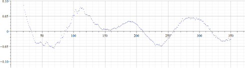
Figure 22.8. Values of “alpha” calculated by using data of Figure 22.7. Parameter “TestDataStep” = 1
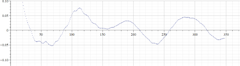
Figure 22.9. Values of “alpha” calculated by using data of Figure 22.7. Parameter “TestDataStep” = 4
Figure 22.7 presents the “total number of Covid-19 deaths per million” for Israel. Figure 22.8 presents the results of calculations of “alpha” for the data presented in Figure 22.7. Parameter “TestDataStep” (as for the previous cases) was set to 1. Figure 22.9 presents the results of calculations of “alpha” for the data presented in Figure 22.7. However, in that case, parameter “TestDataStep” was set to 4. It can be seen that using an increased value of that parameter obviously creates more robust results, albeit decreasing resolution.
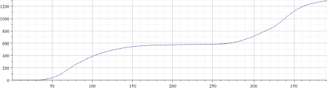
Figure 22.10. Total number of Covid-19 deaths per million (Sweden)
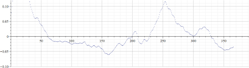
Figure 22.11. Values of “alpha” calculated by using data of Figure 22.10
Figure 22.10 presents the “total number of Covid-19 deaths per million” for Sweden. Figure 22.11 presents the results of calculations of “alpha” for the data presented in Figure 22.10. It can be seen that the behavior of graphs for these two countries differs. Even in the simplest implementation, the proposed method of data approximation by using piecewise exponential functions (parameters of which are effectively changing in time) reveals that well-known parameter: “number of waves” is not as obvious, as it can be seen by visually observing original data. However, more data must be checked to evaluate the usefulness of the proposed method. In addition, different modifications of this method are to be implemented and tested later.
22.5. Conclusion
Analysis of synthetic and real-life Covid-19 data demonstrates that the proposed approach can be used to evaluate the validity of mathematical epidemiological models under test for the different periods of time. Developed equations can be used for the analysis of other processes for which the description by exponents may be adequate. However, more real-life data from different countries must be analyzed in order to recommend an optimal set of the smoothing parameters, and to evaluate the reliability of the proposed approach for the analysis of real-life data.
22.6. References
Kermack, W. and McKendrick, A. (1927). A contribution to the mathematical theory of epidemics. Proceedings of the Royal Society A, 115(772), 700–721.
Okabe, Y. and Shudo, A. (2020). A mathematical model of epidemics – A tutorial for students. Mathematics 2020, 8, 1174 [Online]. Available at: www.mdpi.com/journal/mathematics.
Ritchie, H., Mathieu, E., Rodés-Guirao, L., Appel, C., Giattino, C., Ortiz-Ospina, E., Hasell, J., Macdonald, B., Beltekian, D., Roser, M. (2021). Coronavirus source data, Covid-19 dataset [Online]. Available at: https://ourworldindata.org/coronavirus-source-data.
Wikipedia (n.d.). Compartmental models in epidemiology [Online]. Available at: https://en.wikipedia.org/wiki/Compartmental_models_in_epidemiology.
Chapter written by Samuel KOSOLAPOV.