In this chapter, we present some comprehensive and longer examples together with a brief introduction to the theoretical background and their complete implementation. By this, we want to show you how the concepts defined in this book are used in practice.
First, we will demonstrate the power of the Python constructs presented so far by designing a class for polynomials. We will give some theoretical background, which leads us to a list of requirements, and then we will give the code, with some comments.
Note, this class differs conceptually from the class numpy.poly1d.
A polynomial: p(x) = an x n + an-1 xn-1+…+ a1x + a0 is defined by its degree, its representation, and its coefficients. The polynomial representation shown in the preceding equation is called a monomial representation. In this representation, the polynomial is written as a linear combination of monomials, xi. Alternatively, the polynomial can be written in:
- Newton representation with the coefficients ci and n points, x0, …, xn-1:
p(x) = c0 + c1 (x - x0) + c2 (x - x0)(x-x1) + ... + cn(x - x0) … (x - xn-1)
- Lagrange representation with the coefficients yi and n+1 points, x0, … , xn:
p(x) = y0 l0(x) + y1 l1(x) + … + yn ln(x)
with the cardinal functions:
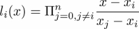
There are infinitely many representations, but we restrict ourselves here to these three typical ones.
A polynomial can be determined from interpolation conditions:
p(xi) = yi i = 0, … , n
with the given distinct values xi and arbitrary values yi as input. In the Lagrange formulation, the interpolation polynomial is directly available, as its coefficients are the interpolation data. The coefficients for the interpolation polynomial in Newton representation can be obtained by a recursion formula, called the divided differences formula:
ci,0 = yi, and
![]() .
.
Finally, one sets ![]() .
.
The coefficients of the interpolation polynomial in monomial representation are obtained by solving a linear system:

A matrix that has a given polynomial p (or a multiple of it) as its characteristic polynomial is called a companion matrix. The eigenvalues of the companion matrix are the zeros (roots) of the polynomial. An algorithm for computing the zeros of p can be constructed by first setting up its companion matrix and then computing the eigenvalues with eig. The companion matrix for a polynomial in Newton representation reads as follows:

We can now formulate some programming tasks:
- Write a class called
PolyNomialwith thepoints,degree,coeff, andbasisattributes, where:pointsis a list of tuples (xi, yi)degreeis the degree of the corresponding interpolation polynomialcoeffcontains the polynomial coefficientsbasisis a string stating which representation is used
- Provide the class with a method for evaluating the polynomial at a given point.
- Provide the class with a method called
plotthat plots the polynomial over a given interval. - Write a method called
__add__that returns a polynomial that is the sum of two polynomials. Be aware that only in the monomial case the sum can be computed by just summing up the coefficients. - Write a method that computes the coefficients of the polynomial represented in a monomial form.
- Write a method that computes the polynomial's companion matrix.
- Write a method that computes the zeros of the polynomial by computing the eigenvalues of the companion matrix.
- Write a method that computes the polynomial that is the ith derivative of the given polynomial.
- Write a method that checks whether two polynomials are equal. Equality can be checked by comparing all coefficients (zero leading coefficients should not matter).