In this chapter, we will give a brief introduction on using Python for symbolic computations. There is powerful software in the market for performing symbolic computations, for example, MapleTM or MathematicaTM. But sometimes, it might be favorable to make symbolic calculations in the language or framework you are used to. At this stage of this book, we assume that this language is Python, so we seek for a tool in Python - the SymPy module.
A complete description of SymPy - if possible, would fill an entire book, and that is not the purpose of this chapter. Instead, we will stake out a path into this tool by some guiding examples, giving a flavor of the potential of this tool as a complement to NumPy and SciPy.
All computations we did so far in this book were so-called numeric computations. These were a sequence of operations mainly on floating-point numbers. It is the nature of numeric computations that the result is an approximation of the exact solution.
Symbolic computations operate on formulas or symbols by transforming them as taught in algebra or calculus into other formulas. The last step of these transformations might then require that numbers are inserted and a numeric evaluation is performed.
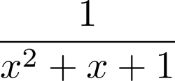
We illustrate the difference by computing this definite integral:

Symbolically this expression can be transformed by considering the primitive function of the integrand:

We now obtain a formula for the definite integral by inserting the integral bounds:
This is called a closed-form expression for the integral. Very few mathematical problems have a solution that can be given in a closed-form expression. It is the exact value of the integral without any approximation. Also no error is introduced by representing real numbers as floating-point numbers, which would otherwise introduce round-off errors.
Approximation and round-off come into play at the very last moment, when this expression needs to be evaluated. The square root and the arctan can only be evaluated approximately by numerical methods. Such an evaluation gives the final result up to a certain (often unknown) precision:
On the other hand, numerical computation would directly approximate the definite integral by some approximation method, for example, Simpson's rule, and deliver a numeric result, often with an estimate of error. In Python, this is done by these commands:
from scipy.integrate import quad
quad(lambda x : 1/(x**2+x+1),a=0, b=4)
They return the value 0.9896614396122965 and an estimate for the error bound 1.1735663442283496 10-08.
The following diagram shows the comparison of numeric and symbolic approximation:

Figure 15.1: Symbolic and numeric quadrature
To begin with, let's elaborate the previous example in SymPy which are explained the steps.
First, we have to import the module:
from sympy import *
init_printing()
The second command makes sure that formulas are presented in a graphical way, if possible. Then, we generate a symbol and define the integrand:
x = symbols('x')
f = Lambda(x, 1/(x**2 + x + 1))
x is now a Python object of type Symbol and f is a SymPy Lambda function (note the command starting with a capital letter).
Now we start with the symbolic computation of the integral:
integrate(f(x),x)
Depending on your working environment, the result is presented in different ways; refer to following screenshot (Figure 15.2) which represents two different result of SymPy formula in different environments:

Figure 15.2: Two screenshots of a SymPy presentation of a formula in two different environments.
We can check by differentiation whether the result is correct. To this end, we assign a name to the primitive function and differentiate with respect to x:
pf = Lambda(x, integrate(f(x),x))
diff(pf(x),x)
The result obtained will be as follows:

which can be simplified by using the following command:
simplify(diff(pf(x),x))
to
 .
.
The result we expected.
The definite integral is obtained by using the following command:
pf(4) - pf(0)
It gives the following output after simplification with simplify:
To obtain a numerical value, we finally evaluate this expression to a floating-point number:
(pf(4)-pf(0)).evalf() # returns 0.9896614396123
