
6
Facial Motion Characteristics
Benjamin ALLAERT1, Ioan Marius BILASCO2 and Chaabane DJERABA2
1IMT Nord Europe, Lille, France
2University of Lille, France
6.1. Introduction
Descriptors based on dense motion characterization (i.e. computation of the motion in each pixel of the image) have proven their efficiency in facial expression analysis, and seem to be better adapted to characterize the dynamics of facial expressions. Although many facial expression analysis processes have been proposed in the literature, it is difficult to find a process as well adapted to characterize low- and high-intensity facial movements. This difficulty is directly related to the motion characteristics of these expressions. In the presence of macro-expressions, facial deformations induced by facial muscles are easily perceptible. However, in the presence of micro-expressions, where the movement intensities are very low, special attention must be paid to encode the subtle deformations.
During the acquisition of faces, the appearance of noise (i.e. motion discontinuities) coming from different factors (illumination, sensor noise, occlusions) reinforces the difficulty of the analysis of facial movements. In addition to the acquisition noise, the analysis of the face is delicate because some facial deformations cause the appearance or disappearance of wrinkles, which cause motion discontinuities. This requires adapting the facial motion characterization process to reinforce the distinction between noise and expression-induced motion. Motion discontinuities complicate motion analysis and significantly reduce the performance of the recognition process.
Recent approaches proposed in the literature directly exploit the information extracted by dense optical flow approaches to characterize facial expressions. However, these approaches do not take into account the specificities of the optical flow approaches used, which are generally not well adapted for facial expression analysis.
To cope with discontinuities, several dense optical flow approaches (e.g. DeepFlow; see Weinzaepfel et al. 2013) have been proposed. However, these approaches are based on generic smoothing and filtering algorithms that do not take into account the specificities of facial motion and require a relatively long computation time. Moreover, the algorithms used to process discontinuities tend to remove relevant information (micro-movements, wrinkles, etc.) related to facial expressions and are therefore not suitable for these applications. Other approaches, such as the one proposed by Farnebäck (2003), makes it possible to compute the dense motion quickly, without reducing the noise induced by the facial features. Although these approaches do not filter noise, they ensure that the extracted data is not modified and that the initial information related to facial expressions is preserved. Non-noise filtering approaches provide a more reliable basis for characterizing facial expressions.
Figure 6.1 represents the computation of the dense optical flow between the two images (A and B) using the Farneback (C) and DeepFlow (D) approaches. Although visually the DeepFlow approach allows us to correct motion discontinuities on the face, we note that some regions devoid of motion have been estimated by smoothing the motion (i.e. the forehead). On the left cheek, we can see that the smoothing has removed the movement induced by the appearance of the wrinkle (which can be seen on the other flow). In this case, there is no guarantee that the estimated information is related to facial expressions. Therefore, to us it seems more interesting to build a model based on a dense unfiltered optical flow, like the one proposed by Farneback, and to add some constraints in order to abstract from the motion discontinuities, and to keep only the information induced by the facial expressions.
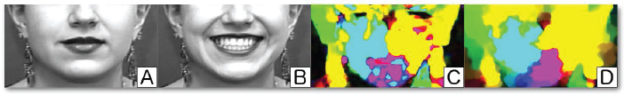
Figure 6.1. Application of Farneback (C) and DeepFlow (D) dense optical flow methods to compute the motion between images A and B.
Inspired by recent uses of motion-based approaches to characterize macro- and micro-expressions, we explore the use of magnitude and orientation constraints to extract only the motion induced by facial expressions. In this chapter, we propose an innovative descriptor called LMP (Local Motion Patterns), which allows us to filter and characterize the motion of facial expressions by freeing us from motion discontinuities. We rely on the specificities of facial motion in order to enhance the characteristics of the movements induced by facial muscles, and to extract the main directions of motion related to facial expressions by freeing ourselves from motion discontinuities.
In the remainder of this chapter, we discuss the specifics of facial movements. More specifically, we analyze the characteristics of motion in the presence of facial expressions, computed using a fast dense motion approach (i.e. Farnebäck 2003). Then, we describe the process for more distinctly dissociating the principal directions associated with facial motion. Finally, we conclude by presenting the contributions of the motion feature filter to characterize a facial motion.
6.2. Characteristics of the facial movement
The extraction of facial motion first requires the study of the specificities of the face. It is therefore important to focus on the deformable properties of biological tissues such as the skin and facial muscles.
The elastic properties of the face imply that expression-induced facial deformation is characterized by a tensile (stretching) or compressive force resulting from facial muscle contraction. The forces exerted by the facial muscles in the presence of facial expressions induce a thermo-dynamic imbalance in the biological tissues of the face. In order to regain thermo-dynamic balance, the skin undergoes deformation. According to the physical laws concerned with the deformation of biological tissues, the following hypotheses can be stated to characterize a facial movement:
1) If we are interested in a small facial region undergoing small deformations, then we can say that the deformation is linear and reversible whatever the constraint. We can therefore assume that there is local consistency in the distribution of motion in terms of magnitude and direction.
2) There are constraints with the application of deformations applied to a solid, according to the shape and material of the solid. It is then possible to consider that the movement of a small region induced by a facial muscle is constrained to follow a principal direction, directly related to the muscle activation.
3) For small deformations, the elongation of an elastic body is proportional to the force applied. In this case, the propagation of the movement within the face is directly proportional to the intensity of a muscle contraction.
4) The thermo-dynamic balance of biological tissues allows us to consider that the magnitude and direction of the deformation propagate continuously in the neighborhood of a facial muscle.
In the remainder of this section, we empirically test whether the different stated hypotheses are verified when characterizing a facial movement. For each of these hypotheses, we analyze several motion distributions extracted from different facial regions. The facial motion is computed using the dense optic flow method proposed by Farnebäck (2003). Contrary to recent dense optical flow methods, this method does not include any preprocessing (e.g. smoothing) that can modify the extracted information. Moreover, this solution has the particularity of being very fast. The analyses are performed in the presence of facial deformations induced, on the one hand, by macro-expressions, and, on the other hand, by micro-expressions.
6.2.1. Local constraint of magnitude and direction
In this section, we focus on the local consistency of motion distribution in terms of magnitude and direction. Specifically, we analyze the correlation between the direction and magnitude of motion in the presence of a facial expression. Under hypothesis A, a facial deformation is linear, which implies that there is local coherence of the motion distribution in terms of magnitude and direction. Otherwise, the consistency of the local motion is not guaranteed.
In order to test hypothesis A, we analyze the facial deformation induced by the facial muscles in the presence of a smile (lip corner elevation). Figure 6.2 illustrates the local motion distribution extracted from different regions of the face. The distributions are computed from the dense optical flow algorithm proposed by Farnebäck (2003). In this analysis, the dimension of the regions (parameter λ) corresponds to 3% of the size of the face analyzed, which corresponds here to regions of dimension 15×15 pixels, either for the macro- or the micro-expression.
The distribution of the direction of the movement is analyzed on several layers of magnitudes. The magnitude layers vary from 0 to 10, with a step of 0.2 between each layer (50 magnitude layers). We decided not to consider magnitudes going beyond 10, given the average size of the faces contained in the analyzed databases. This interval has shown its efficiency to characterize equally the macro (recording rate of 25 fps) and micro (recording rate of 100–200 fps) expressions. Like the different parameters of the descriptor proposed in the following section, this value can be modulated according to the size of the face and/or the recording rate of the video. Currently, the amplitude of 10 pixels characterizing the maximum magnitude corresponds to 2% of the average face diagonal. In Figure 6.2, the higher the magnitude, the more red the associated curve. The blue curve represents the total motion distribution without magnitude filtering. The abscissa represents the direction, divided into 36 bins (10° per bin). The ordinate represents the number of occurrences of the pixels within the distribution (%).
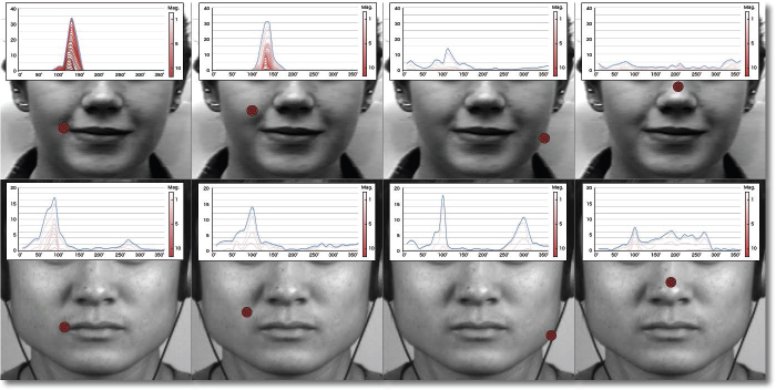
Figure 6.2. Analysis of the motion distribution on different magnitude scales, in the presence of a macro- (first line – CK+) and a micro- (second line – CASME II) expression (smile).
The first column of Figure 6.2 represents the localized motion distribution at the lip corner. In the presence of a macro-expression (first row of Figure 6.2), we note a significant succession of magnitude layers converging in a common direction. We make the same observation in the presence of a micro-expression (second line of Figure 6.2), with the only difference being the number of layers of magnitudes. This can be explained by the fact that a micro-expression is less intense than a macro-expression. From these two distributions, we can identify that the main direction of motion tends to remain the same across the different magnitude layers.
The second column of Figure 6.2 represents the distribution of motion in a region near the corner of the lips. We always note the same behavior, both in the presence of macro- and micro-expressions. As the distribution is further away from the epicenter of the motion, the magnitude is lower. This is also illustrated by the fact that the number of layers of magnitudes is less important. We note in this case that the gap between successive layers tends to increase, which shows that the linearity of the local motion tends to decrease.
The last two columns of Figure 6.2 represent motion distributions extracted in regions not affected by lip wedge motion. We note in this case that the motion distribution tends to be more heterogeneous. This implies that the main direction of motion does not stand out as much as before. Sometimes, the main direction stands out very clearly in the distribution, this is the case in column three, corresponding to the micro-expression. In this case, it is important to note that the number of magnitude layers is small and that the different magnitude layers converging in the same direction are widely spaced. This means that the linearity of the local motion is no longer guaranteed.
From the different distributions, we can conclude that a muscle-induced facial deformation is characterized by a linear motion, where direction and magnitude are correlated. In this case, the main direction is characterized by a continuous progression of orientation over several magnitude levels, which validates hypothesis A. The coherence of the local motion can be assessed by the successive convergence of the different magnitude layers in the same direction. The greater the number of magnitude layers and the smaller the gap between them, the more likely the motion is locally coherent.
The correlation between direction and magnitude is a criterion to consider when characterizing a facial motion. However, this criterion alone is not always sufficient to ensure that the principal direction reflects a coherent motion. This is particularly the case when the motion distribution is heterogeneous and the facial motion tends to be confused with noise (motion discontinuity, acquisition noise). In this case, it is important to verify a second coherence criterion based on the constraints related to the shape and material of a deformable solid (hypothesis B). In the following section, we propose an analysis to verify this criterion.
6.2.2. Local constraint of the motion distribution
In this section, we are interested in the distribution of the direction of facial motion within a small region. More specifically, we verify that hypothesis B, which states that the local deformation of a solid is directly related to its shape and material, applies well to the face.
In the case of a facial deformation, we need to identify how the skin deformation manifests itself according to the movement induced by a facial muscle. To do this, we use the same facial regions as before, but here we only analyze the direction of the total pixel distribution within a region (15×15 pixels), without taking into account the magnitude. Figure 6.3 illustrates the set of motion distributions induced by a macro (first line) and a micro (second line) expression. The distributions are calculated from the dense optical flow algorithm proposed by Farnebäck (2003). For the distributions, the abscissa represents the direction, divided into 36 bins (10° per bin), and the ordinate represents the number of occurrences of the pixels within the distribution (in percent).
The first two columns of Figure 6.3 represent the motion distributions extracted in regions near the epicenter of the motion. We note that the motion distribution around the main direction tends to spread out and progressively decrease on the neighboring directions. The observation is the same whether in the presence of a macro (first line) or a micro (second line) expression. This shows that the local deformation progressively converges towards a main direction.
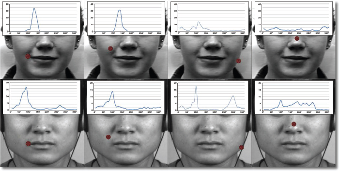
Figure 6.3. Analysis of the distribution of facial motion direction within the distribution, in the presence of a macro (first line – CK+) and micro (second line – CASME II) expression (smile).
Concerning the last two columns of Figure 6.3, where no expression-induced motion is observable, we distinguish several categories of distributions:
– In some regions, the distribution extends in all directions with very low intensity. In this case, the information contained in the distribution is not important enough to characterize a facial deformation. The small variations observed are generally due to acquisition noise.
– In other cases, a wide spread in terms of significant distribution can be observed, as in the last column of the second row. It is then important to check whether the motion represented by the distribution is relevant to the specifics of the facial deformations. If we consider that we are analyzing small regions, there is a good chance that the main direction does not spread beyond a certain threshold (∈ [0°–60°]).
– Sometimes a main direction is characterized by a high concentration in a single direction. This is notably the case in the third column of the second row. This high concentration is usually observed in the presence of motion discontinuities, mainly at the edges. This is due to the fact that the motion vectors associated with the contour pixels tend to be poorly estimated due to occlusions. In this case, there is no continuity of motion around the main direction, which results in a very strong variation between two different directions within the distribution.
From these distributions, we note that the motion within a small region is constrained to cover a fairly small range of directions (related to the applied force) while maintaining some consistency in the convergence of directions. It is then important to ensure that the main directions remain consistent in terms of intensity, variation and overlap, to conform to the physical constraints characterizing a facial deformation.
So far, we have discussed several criteria for ensuring consistency of motion within a small region. However, the force applied in the presence of a facial expression generally implies that the deformation propagates beyond the region containing the epicenter of the motion. In the next section, we analyze how motion induced by a facial deformation propagates.
6.2.3. Motion propagation constraint
In this section, we are interested in the propagation of facial motion within a small region (15×15 pixels). More specifically, we test hypotheses C and D related to the elastic characteristics of the facial skin. The objective is to verify if the main direction of motion within different neighboring regions remains consistent despite the distance between them and the corner of the lips.
Figure 6.4 shows the distributions extracted from three regions located at different distances from the lip corner. The distributions are calculated from the dense optical flow algorithm proposed by Farnebäck (2003). The last column groups the three distributions together to easily compare the overlap between the main directions. For the distributions, the abscissa represents the direction, divided into 36 bins (10° per bin), and the ordinate represents the number of occurrences of the pixels within the distribution (as a percentage).
Looking at the different distributions concerning the macro-expression (Figure 6.4, first row), we note a strong correspondence between the main directions despite the distance between the lip corner regions. This shows that the deformation propagates continuously in the neighborhood of a facial muscle in the presence of a high intensity movement. However, the greater the distance to the epicenter of motion, the more the principal direction diverges to other bins.
Concerning the micro-expression (Figure 6.4, second row), we note the same behavior. On the contrary, the muscular intensity being lower, the propagation of the movement is less important. This is illustrated in the distribution of the third column, where the main direction of the movement induced by the corner of the lips is no longer as clearly distinguishable.
From these results, we can conclude that the propagation of motion within the face appears to be related to the elastic properties of the skin, and is directly proportional to the intensity of a muscle contraction. This confirms that hypotheses C and D apply in the context of facial movements. Facial deformation thus implies that there is consistency in magnitude and direction of motion between two neighboring regions.
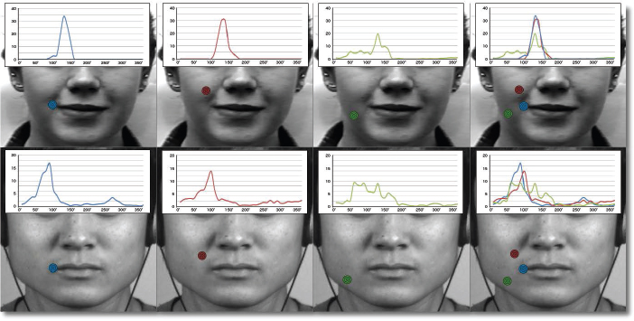
Figure 6.4. Analysis of motion propagation around the corner of the lips, in the presence of a macro (first line – CK+) and a micro (second line – CASME II) expression (smile).
In the following section, we summarize the different hypotheses related to the specificities of the face. From these hypotheses, we propose a motion characterization process adapted to the deformations of a solid such as the face.
Given the hypotheses related to facial motion, the characterization of facial motion is done at two different levels of analysis. The validation of hypotheses A and B consists of analyzing the veracity of a movement within a small region, ensuring that there is a local coherence of the movement as a function of the force applied. Hypotheses C and D validate the coherence of the motion by ensuring that it is reflected in the neighborhood of the epicenter. Although the experiments presented in this section only focused on the behavior of the movement around the facial muscle of the mouth, it is important to note that the same behavior applies to the other muscles of the face. We consider that the principal directions of facial motion must satisfy all of these constraints in order to more distinctly dissociate facial motion from noise.
Based on these different hypotheses, we propose a process of characterization of the facial movement allowing us to extract only the main directions and to abstract noise (acquisition noise, discontinuity of the movement). An illustration of the different steps of the filtering and motion characterization process is presented in Figure 6.5. Each region is analyzed locally to check if the local motion distribution is consistent with the observed facial deformation (Figure 6.5-1 (hypothesis A) and Figure 6.5-2 (hypothesis B)). In the case where the motion is locally coherent, the analysis is applied to a related region to ensure that the motion propagates correctly in its neighborhood (Figure 6.5-3 (hypothesis C and D)). If any of the steps in the process fail, then the analyzed motion is not associated with a true facial deformation.
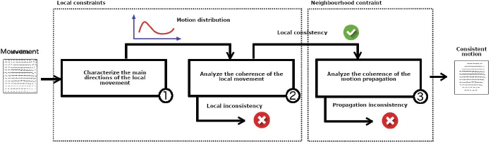
Figure 6.5. Scheme of the filtering process for motion characterization.
In the following section, we detail the process of filtering and characterizing facial motion called LMP based on the process defined in Figure 6.5.
6.3. LMP
Facial characteristics (skin elasticity and reflectance, smooth texture) induce inconsistencies and noise in the facial motion extraction process. We rely on the specificities of the facial movement to enhance the characteristics of the movements induced by the facial muscles. In view of the facial characteristics, we consider that a natural movement implies a certain local coherence (no discontinuity) and must propagate continuously around the neighboring regions.
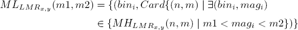
To take into account these motion constraint hypotheses, and extract coherent motion from a specific facial region, we propose a new descriptor called LMP. An LMP filters out noise and characterizes the main directions of motion within a region, locally verifying the motion propagation constraint in a region. Each region defined with respect to its center C(x,y), called LMR (Local Motion Region), is characterized by an optical flow histogram ![]() We define two types of LMRs:
We define two types of LMRs:
– The central region (which assumes the main direction that the motion will take within the LMP) is called CMR (Central Motion Region). This region allows us to determine the nature of the motion at the epicenter of the LMP in order to anticipate the propagation on the neighboring regions.
– The neighboring regions around the epicenter are called NMR (Neighboring Motion Region). They allow us to analyze the motion propagation and to quantify the coherence of the motion with respect to the main direction defined within the CMR.
A representation of the LMP is given in Figure 6.6. Eight NMRs are generated around the CMR. All regions are placed at a distance Δ from the CMR. The distance defined by Δ represents the level of overlap between two neighboring regions. The variable λ defines the dimension of a region, where each region covers λ × λ pixels. Finally, the variable β defines the number of direct propagations from the epicenter to check the consistency of the motion propagation in the neighboring regions.
In the subsequent section, we present in detail the methodology to extract the relevant motion on a face, based on the characteristics of the face, and the motion constraints induced by the facial muscles.
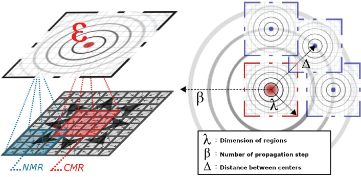
Figure 6.6. General view of the structure of an LMP.
6.3.1. Local consistency of the movement
In order to filter the facial motion, we first analyze the motion distribution within a CMR. The objective is to keep only the relevant motion contained in the information returned by the optical flow. To do so, we propose to extract only the motion of the main directions while abstracting from the noise (acquisition noise, motion discontinuity). The first step of the process is to calculate the distribution of the motion of a small region on several layers of magnitudes. Then, for each direction, we calculate the number of occurrences of the same direction at different magnitude levels. Finally, we weight the motion distribution according to these different magnitude levels for each direction. This allows us to obtain a new distribution containing only the main directions of the motion, with a focus on strong coherence in terms of magnitude. Each of these steps is detailed in the rest of this section.
6.3.1.1. [Step 1] :
Like all regions within the LMP, a CMR is an LMR and is defined by a location (x,y). An LMR is characterized by a histogram of direction ![]() of size B bins (distribution in B direction classes). The motion distribution of the LMR is divided into q histograms corresponding to different magnitude layers. This splitting allows a more detailed analysis of the local motion. The multi-layer analysis of the motion magnitude allows us to identify low- and high-intensity motions that occur on several successive layers. Each LMR magnitude layer is defined as follows:
of size B bins (distribution in B direction classes). The motion distribution of the LMR is divided into q histograms corresponding to different magnitude layers. This splitting allows a more detailed analysis of the local motion. The multi-layer analysis of the motion magnitude allows us to identify low- and high-intensity motions that occur on several successive layers. Each LMR magnitude layer is defined as follows:
[6.1]
where n and m represent the magnitude intervals and i = 1, 2, ..., Bin is the index of direction bins (classes). The distribution of the motion by magnitude layers ![]() a macro- and a micro-expression is shown in Figure 6.7. In this case, we have varied the parameter n from 0 to 10, by steps of 0.2. As for the parameter m, it is fixed at 10 in order to guarantee an overlap of the different layers of magnitudes. The successive layers of magnitudes make it possible to easily distinguish the main directions.
a macro- and a micro-expression is shown in Figure 6.7. In this case, we have varied the parameter n from 0 to 10, by steps of 0.2. As for the parameter m, it is fixed at 10 in order to guarantee an overlap of the different layers of magnitudes. The successive layers of magnitudes make it possible to easily distinguish the main directions.
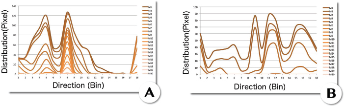
Figure 6.7. Representation of the motion distribution by magnitude layer of a macro- (A) and micro- (B) expression.
6.3.1.2. [Step 2] :
Each ![]() is then normalized. Directions with a magnitude less than 10% are filtered out (set to 0). Each distribution is then divided into three intervals P1 ∈ (0%, 33%], P2 ∈]33%, 66%], and P3 ∈]66%, 100%], represented by three cumulative histograms
is then normalized. Directions with a magnitude less than 10% are filtered out (set to 0). Each distribution is then divided into three intervals P1 ∈ (0%, 33%], P2 ∈]33%, 66%], and P3 ∈]66%, 100%], represented by three cumulative histograms ![]() calculated as follows:
calculated as follows:
[6.2]
The different intervals thus allow us to dissociate the directions with low, medium and high representativeness across the magnitude levels. Thanks to this, we can apply a weighting factor to the different levels of direction co-occurrence across the magnitudes, allowing us to favor certain directions over others. Figure 6.8 represents the division of the ![]() by the three intervals P1, P2 and P3. Each
by the three intervals P1, P2 and P3. Each ![]() corresponds to a row in the table and the number in each cell represents the number of occurrences of each magnitude for each direction.
corresponds to a row in the table and the number in each cell represents the number of occurrences of each magnitude for each direction.
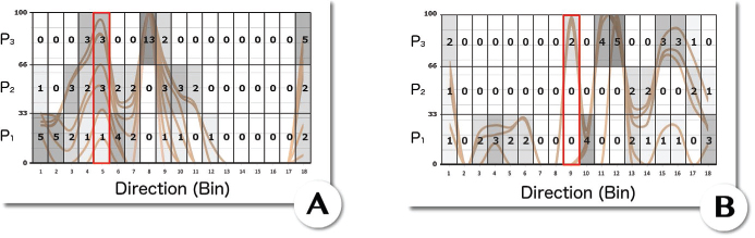
Figure 6.8. Division of  based on three magnitude intervals. (A) macro- and (B) micro-expression.
6.3.1.3. [Step 3] :
The magnitude and direction histogram ![]() is calculated by applying different weighting factors ω1, ω2 and ω3, to each cumulative histogram
is calculated by applying different weighting factors ω1, ω2 and ω3, to each cumulative histogram ![]() is defined by the following equation:
is defined by the following equation:

This equation allows us to reinforce the local coherence of the magnitude in each direction. We applied a factor of 10 between each layer (ω1 = 1, ω2 = 10 and ω3 = 100). The values associated with the three factors can vary depending on what we want to quantify in the local motion analysis. In this case, the higher the co-occurrence of a direction across the magnitudes, the higher the associated weight. This allows us to give more weight to a motion that has a constant magnitude between several layers. A representation of the ![]() direction and magnitude histograms of the previous two examples is shown in Figure 6.9.
direction and magnitude histograms of the previous two examples is shown in Figure 6.9.
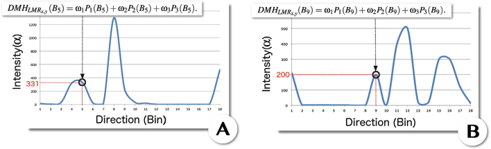
Figure 6.9. Calculation of direction and magnitude histograms. (A) macro- and (B) micro-expression.
At this stage of the process, we obtain a new motion distribution, where only the main directions appear. Now we have to check if these directions are consistent with the facial deformation specificities. In the next section, we present the second step of the motion feature filtering process within the LMP.
6.3.2. Consistency of local distribution
In order to verify the facial motion hypotheses, the histogram of magnitudes and directions of the LMR (![]() ) must contain at least one principal direction consistent with the specifics of the facial deformations. To do this, we check that the distribution of the LMR (
) must contain at least one principal direction consistent with the specifics of the facial deformations. To do this, we check that the distribution of the LMR (![]() ) contains at least one principal direction that verifies the following three criteria:
) contains at least one principal direction that verifies the following three criteria:
– the intensity of the movement is high enough;
– the main movement does not propagate in all directions;
– the movement gradually converges towards the main direction.
6.3.2.1. [Step 1] :
To identify the principal directions within a distribution, we apply a thresholding α on the value of the co-occurrence of a direction across the magnitude levels. The threshold α depends mainly on the associated weights in the equation [6.3]. If no direction is sufficiently intense, it means that the local motion is not sufficiently distinguishable from the noise in the epicenter region of the LMP. In this case, we consider that the CMR representing the LMP does not contain significant information, which implies that the analysis within the LMP will not be deepened.
6.3.2.2. [Step 2] :
In the case where at least one principal direction is found, it is necessary to ensure that the directions selected within the ![]() represent coherent movements for a face. Indeed, a movement can be consistent in terms of magnitude, but we must also make sure that it is consistent in terms of direction. More specifically, the main direction of the motion cannot cover a large range of directions within a small region of the face. This step ensures that a consistent and selective framework is maintained for the motion propagation analysis.
represent coherent movements for a face. Indeed, a movement can be consistent in terms of magnitude, but we must also make sure that it is consistent in terms of direction. More specifically, the main direction of the motion cannot cover a large range of directions within a small region of the face. This step ensures that a consistent and selective framework is maintained for the motion propagation analysis.
To ensure that the motion is consistent in terms of direction, we analyze the density of the k principal directions of the ![]() . Each principal direction must satisfy several criteria. The first criterion verifies that each principal direction extends over a limited scattering angle. Indeed, if we analyze a small facial region, a coherent motion rarely extends over a wide range of direction bins and the spread of the motion is progressive around the principal direction. If no principal direction validates this criterion, then the motion within the CMR is inconsistent, and the LMP analysis is stopped. Despite the coherence of the motion in terms of magnitude, a direction covering a large enough angle has a high chance of corresponding to a false motion, and can lead to errors in the propagations within the LMP. The criterion is defined by the following equations. The first equation is used to calculate the spread of a main direction, while the second equation is used to check whether these intervals respect the tolerated limit:
. Each principal direction must satisfy several criteria. The first criterion verifies that each principal direction extends over a limited scattering angle. Indeed, if we analyze a small facial region, a coherent motion rarely extends over a wide range of direction bins and the spread of the motion is progressive around the principal direction. If no principal direction validates this criterion, then the motion within the CMR is inconsistent, and the LMP analysis is stopped. Despite the coherence of the motion in terms of magnitude, a direction covering a large enough angle has a high chance of corresponding to a false motion, and can lead to errors in the propagations within the LMP. The criterion is defined by the following equations. The first equation is used to calculate the spread of a main direction, while the second equation is used to check whether these intervals respect the tolerated limit:
[6.4]
[6.5]
where a and b represent the limits of the spread of a principal direction and α, the magnitude threshold. For each principal direction, we keep only the motions spreading over s consecutive bins, at most.
6.3.2.3. [Step 3] :
To reinforce the fact that the movement spreads progressively around a direction, it is important to check that the transition between the different successive bins is progressive. A Φ tolerance is accepted between the different bins. The criterion is validated by the following equation:
[6.6]
Finally, the filtered histogram of directions and magnitudes ![]() corresponds to the k principal directions extracted from the
corresponds to the k principal directions extracted from the ![]() , each one satisfying the previously mentioned criteria. The histogram of the
, each one satisfying the previously mentioned criteria. The histogram of the ![]() is described by the following equation:
is described by the following equation:
[6.7]
Although the motion within the CMR is consistent, the compliance of the motion within the LMP is not yet verified. Although the epicenter of the motion allows us to identify potential principal directions, we need to ensure that they propagate correctly in their neighborhood. The analysis of the motion propagation within the LMP is detailed in the next section.
6.3.3. Coherence in the propagation of the movement
When the motion distribution of an LMP is consistent within its CMR (epicenter of motion), it should be verified that the calculated motion propagates correctly in its neighborhood. Indeed, the elasticity of the skin ensures that a facial motion propagates on the face in a progressive and continuous way. In this case, the coherence of the movement in terms of intensity and direction within the neighboring regions must be respected to ensure that it is not noisy. The fact that the face is a non-rigid element implies that the direction and magnitude of the motion may undergo gradual deformation during propagation.
Before checking the coherence of the motion propagation, it is important to ensure the local coherence of the motion within each NMR. As a reminder, each NMR is represented by an LMR, which means that each NMR is characterized by a filtered histogram of directions and magnitudes ![]() . As with the CMR, the local motion within each NMR must be consistent in terms of magnitude and directions.
. As with the CMR, the local motion within each NMR must be consistent in terms of magnitude and directions.
In addition to ensuring consistency of distribution within an NMR, it is important to verify that there is a correlation in terms of the principal directions of the NMR with respect to the principal directions characterizing the CMR. This step in the process verifies hypothesis C, which states that motion propagates as a function of skin elasticity stress. For this, the Bhattacharyya coefficient (Bhattacharyya 1943) is employed to determine the relative proximity of two motion distributions. The Bhattacharyya coefficient is calculated as follows:
[6.8]
where ![]() and
and ![]() represent the two local distributions and B the number of bins. The coherence of the motion between the two adjacent regions is ensured if the coefficient is greater than a fixed threshold ρ.
represent the two local distributions and B the number of bins. The coherence of the motion between the two adjacent regions is ensured if the coefficient is greater than a fixed threshold ρ.
A representation of the motion propagation analysis within an LMP is shown in Figure 6.10. The figure shows the first iteration of the motion analysis around the CMR, i.e. the propagation of motion from the CMR to the eight adjacent NMRs. The coherence of an NMR is measured with several criteria:
– the distribution of motion within the NMR in terms of magnitude;
– the distribution of movement within the NMR in terms of direction;
– the similarity index between the motion distributions of two related regions.

Figure 6.10. Calculation of the distribution of the LMP motion within the direct neighborhood of the CMR (first iteration).
If these three criteria are verified, a binary coherence map is updated to keep track of the coherent regions and avoid reprocessing them in subsequent iterations. In the instance where the motion distribution of an NMR is inconsistent, it can be re-evaluated and checked against another adjacent region during the next iterations of the analysis. This is notably the case in the presence of motion discontinuity associated with the appearance or disappearance of a wrinkle, where in this case, the motion can be indirectly linked to its neighborhood by bypassing the disturbing element.
Then, recursively, for each NMR verifying the three coherence criteria, the motion propagation analysis is reiterated to its neighborhood. The recursive analysis is reiterated as long as there is a coherence of motion with at least one adjacent region, or as long as the desired number of iterations is reached (the number of propagations is defined by the parameter β of the LMP).
If no motion coherence between the CMR and the eight adjacent NMRs is found, then this means that there is no motion testing hypotheses C and D of a facial motion in the region characterizing the LMP.
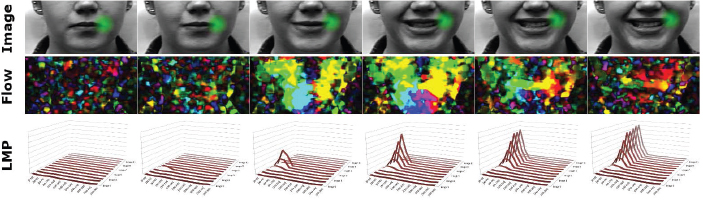
Figure 6.11. Application of LMP to characterize coherent facial motion around the corner of the lips (green region) (CK+).
In the case where several adjacent regions are coherent, then the motion distributions (![]() ) of the NMRs with a direct or indirect correspondence to the local CMR motion are cumulated to characterize the motion within the LMP. The LMP motion distribution is calculated as follows:
) of the NMRs with a direct or indirect correspondence to the local CMR motion are cumulated to characterize the motion within the LMP. The LMP motion distribution is calculated as follows:
[6.9]

where n represents the number of regions where the local motion distribution is coherent (the CMR and the set of coherent NMRs). In the case of an eight related analysis (eight neighboring regions), the maximum number that n can reach can be calculated by the following equation:
[6.10]
where β represents the number of iterations. The LMP motion distribution ![]() is characterized by a histogram of B bins, where the value of each bin is the sum of the different histograms (
is characterized by a histogram of B bins, where the value of each bin is the sum of the different histograms (![]() ) of each region where the local motion is coherent. At this stage of the process, we can compute the coherent motion of a specific facial region defined by an LMP.
) of each region where the local motion is coherent. At this stage of the process, we can compute the coherent motion of a specific facial region defined by an LMP.
An application of the motion feature filtering is illustrated in Figure 6.11. An LMP is placed on a face to characterize the coherent facial motion. The LMP is characterized by a histogram of directions (decomposed into 12 bins in the example) representing the distribution of motion that spans the facial region, having coherence with the epicenter represented by the green region. The LMP is directly characterized from the optical flow computed by the Farnebäck method (Farnebäck 2003) (second row). Although the optical flow is highly noisy throughout the sequence, the LMP allows us to keep only the coherent motion (line 3).
6.4. Conclusion
In this chapter, we proposed a new descriptor based on facial features to filter the acquisition noise and motion discontinuities caused by different factors (illumination, sensor noise, occlusions). The proposed filtering makes it possible to keep only the information related to facial expressions of variable intensity, based on the motion computed by a fast dense optical flow method.
In order to identify and understand the specifics of facial motion, we first analyzed facial motion behavior by analyzing several facial regions locally. To analyze the facial motion behavior, we used a fast dense motion approach (i.e. Farnebäck 2003) to extract the facial motion. The local distribution of these regions allowed us to identify several hypotheses regarding the natural behavior of a facial movement. Facial characteristics such as skin elasticity and muscle constraints imply that motion propagates continuously within the face, while maintaining consistency in direction and magnitude. Based on these hypotheses, we proposed a new motion feature filter called LMP, allowing us to keep only the motion validating the facial specificities.
The motion feature filtering proposed within LMP tests three hypotheses to ensure that the local motion is representative of facial motion. The different steps in the filtering process verify that there is: (a) convergence between different magnitude layers in the same direction, (b) that the local motion distribution characterizes one or more principal directions and (c) that there is consistency in the motion propagation. These three criteria are based directly on the hypotheses made in terms of the characteristics associated with facial motion. This ensures that the motion extracted within the LMP is consistent with a motion that is coherent with respect to the specifics of the face.
In this approach, instead of explicitly computing the motion on the whole face, the motion is computed in specific regions in order to keep only the motions induced by the facial expressions. These regions are defined in relation to the FACS system and allow us to directly analyze the coherent movements induced by facial muscles. We then exploited the motion coherence hypothesis and improved the distinction between motion-related information and noise present in the data.
In view of the different steps in the filtering process, we have seen that the LMP allows us to simultaneously characterize a facial movement with a low- or high- intensity magnitude. Each evaluation criterion of the filtering process can be configured independently from the other criteria, which makes the LMP fully adaptable. To verify the performance of the descriptor, in the next chapter we analyze the robustness of the LMP for macro- and micro-expression recognition.
6.5. References
- Bhattacharyya, A. (1943). On a measure of divergence between two statistical populations defined by their probability distributions. Bulletin of the Calcutta Mathematical Society, 35, 99–109.
- Farnebäck, G. (2003). Two-frame motion estimation based on polynomial expansion. Image Analysis: 13th Scandinavian Conference, SCIA 2003, 363–370.
- Weinzaepfel, P., Revaud, J., Harchaoui, Z., Schmid, C. (2013). Deepflow: Large displacement optical flow with deep matching. IEEE International Conference on Computer Vision (ICCV), 1385–1392.