1

Getting Started with Time Series Analysis

When embarking on a journey to learn coding in Python, you will often find yourself following instructions to install packages and import libraries, followed by a flow of a code-along stream. Yet an often-neglected part of any data analysis or data science process is ensure that the right development environment is in place. Therefore, it is critical to have the proper foundation from the beginning to avoid any future hassles, such as an overcluttered implementation or package conflicts and dependency crisis. Having the right environment setup will serve you in the long run when you complete your project, ensuring you are ready to package your deliverable in a reproducible and production-ready manner.

Such a topic may not be as fun and may feel administratively heavy as opposed to diving into the core topic or the project at hand. But it is this foundation that differentiates a seasoned developer from the pack. Like any project, whether it is a machine learning project, a data visualization project, or a data integration project, it all starts with planning and ensuring all the required pieces are in place before you even begin with the core development.

In this chapter, you will learn how to set up a Python virtual environment, and we will introduce you to two common approaches for doing so. These steps will cover commonly used environment management and package management tools. This chapter is designed to be hands-on so that you avoid too much jargon and can dive into creating your virtual environments in an iterative and fun way.

As we progress throughout this book, there will be several new Python libraries that you will need to install specific to time series analysis, time series visualization, machine learning, and deep learning on time series data. It is advised that you don't skip this chapter, regardless of the temptation to do so, as it will help you establish the proper foundation for any code development that follows. By the end of this chapter, you will have mastered the necessary skills to create and manage your Python virtual environments using either conda or venv.

The following recipes will be covered in this chapter:

• Development environment setup
• Installing Python libraries
• Installing JupyterLab and JupyterLab extensions

Technical requirements

In this chapter, you will be primarily using the command line. For macOS and Linux, this will be the default Terminal (bash or zsh), while on a Windows OS, you will use the Anaconda Prompt, which comes as part of the Anaconda installation. Installing Anaconda will be discussed in the following Getting ready section.

We will use Visual Studio Code for the IDE, which is available for free at https://code.visualstudio.com. It supports Linux, Windows, and macOS.

Other valid alternative options that will allow you to follow along include the following:

• Sublime Text 3 at https://www.sublimetext.com/3
• Atom at https://atom.io/
• PyCharm Community Edition at https://www.jetbrains.com/pycharm/download/

The source code for this chapter is available at https://github.com/PacktPublishing/Time-Series-Analysis-with-Python-Cookbook.

Development environment setup

As we dive into the various recipes provided in this book, you will be creating different Python virtual environments to install all your dependencies without impacting other Python projects.

You can think of a virtual environment as isolated buckets or folders, each with a Python interpreter and associated libraries. The following diagram illustrates the concept behind isolated, self-contained virtual environments, each with a different Python interpreter and different versions of packages and libraries installed:

Figure 1.1 – An example of three different Python virtual environments, one for each Python project

These environments are typically stored and contained in separate folders inside the envs subfolder within the main Anaconda folder installation. For example, on macOS, you can find the envs folder under Users/<yourusername>/opt/anaconda3/envs/. On Windows OS, it may look more like C:Users<yourusername>anaconda3envs.

Each environment (folder) contains a Python interpreter, as specified during the creation of the environment, such as a Python 2.7.18 or Python 3.9 interpreter.

Generally speaking, upgrading your Python version or packages can lead to many undesired side effects if testing is not part of your strategy. A common practice is to replicate your current Python environment to perform the desired upgrades for testing purposes before deciding whether to move forward with the upgrades. This is the value that environment managers (conda or venv) and package managers (conda or pip) bring to your development and production deployment process.

Getting ready

In this section, it is assumed that you have the latest Python version installed by doing one of the following:

• The recommended approach is to install through a Python distribution such as Anaconda (https://www.anaconda.com/products/distribution), which comes preloaded with all the essential packages and supports Windows, Linux, and macOS (including M1 support as of version 2022.05). Alternatively, you can install Miniconda (https://docs.conda.io/en/latest/miniconda.html) or Miniforge (https://github.com/conda-forge/miniforge).
• Download an installer directly from the official Python site https://www.python.org/downloads/.
• If you are familiar with Docker, you can download the official Python image. You can visit Docker Hub to determine the desired image to pull https://hub.docker.com/_/python. Similarly, Anaconda and Miniconda can be used with Docker by following the official instructions here : https://docs.anaconda.com/anaconda/user-guide/tasks/docker/

At the time of writing, the latest Python version that's available is Python 3.10.4.

Latest Python Version Supported in Anaconda

The latest version of Anaconda, 2022.05, released on May 6, 2022, supports the latest version of Python 3.10.4. By default, Anaconda will implement Python 3.9.12 as the base interpreter. In addition, you can create a Python virtual environment with Python version 3.10.4 using conda create, which you will see later in this recipe.

The simplest and most efficient way to get you up and running quickly and smoothly is to go with a Python distribution such as Anaconda or Miniconda. I would even go further and recommend that you go with Anaconda.

If you are a macOS or Linux user, once you have Anaconda installed, you are pretty much all set for using your default Terminal. To verify the installation, open your Terminal and type the following:

$ conda info

The following screenshot shows the standard output when running conda info, which outlines information regarding the installed conda environment. You should be interested in the listed versions for both conda and Python:

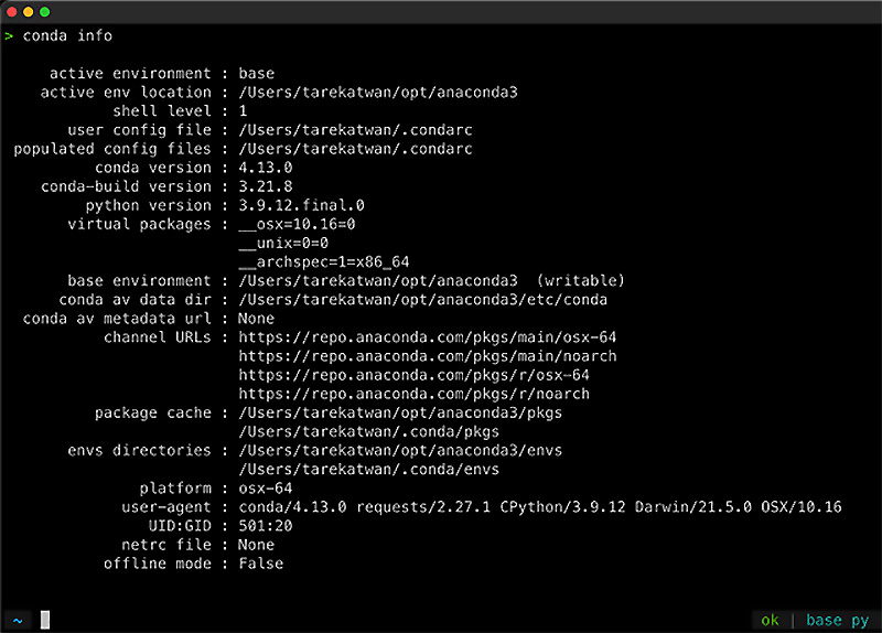
Figure 1.2 – Verifying Conda's installation on macOS using the Terminal

If you installed Anaconda on a Windows OS, you need to use Anaconda Prompt. To launch it, you can type Anaconda in the Windows search bar and select one of the Anaconda Prompts listed (Anaconda Prompt or Anaconda PowerShell Prompt). Once Anaconda Prompt has been launched, you can run the conda info command.

How to do it…

In this recipe, I will cover two popular environment management tools. If you have Anaconda, Miniconda, or Miniforge installed, then conda should be your preferred choice since it provides both package dependency management and environment management for Python (and supports many other languages). On the other hand, the other option is using venv, which is a Python module that provides environment management, comes as part of the standard library in Python 3, and requires no additional installation.

Both conda and venv allow you to create multiple virtual environments for your Python projects that may require different Python interpreters (for example, 2.7, 3.8, or 3.9) or different Python packages. In addition, you can create a sandbox virtual environment to experiment with new packages to understand how they work without affecting your base Python installation.

Creating a separate virtual environment for each project is a best practice taken by many developers and data science practitioners. Following this recommendation will serve you well in the long run, helping you avoid common issues when installing packages, such as package dependency conflicts.

Using Conda

Start by opening your terminal (Anaconda Prompt for Windows):

1. First, let's ensure that you have the latest conda version. This can be done by using the following command:

   conda update conda

The preceding code will update the conda package manager. This is helpful if you are using an existing installation. This way, you make sure you have the latest version.

2. If you have Anaconda installed, then you can update to the latest version using the following command:

   conda update anaconda
3. You will now create a new virtual environment named py39 with a specific Python version, which in this case, is Python 3.9:

   $ conda create -n py39 python=3.9

Here, -n is a shortcut for --name.

4. conda may identify additional packages that need to be downloaded and installed. You may be prompted on whether you want to proceed or not. Type y and then hit Enter to proceed.
5. You could have skipped the confirmation message in the preceding step by adding the -y option. Use this if you are confident in what you are doing and do not require the confirmation message, allowing conda to proceed immediately without prompting you for a response. You can update your command by adding the -y or --yes option, as shown in the following code:

   $ conda create -n py39 python=3.9 -y
6. Once the setup is complete, you will be ready to activate the new environment. Activating a Python environment means that our $PATH environment variable will be updated to point to the specified Python interpreter from the virtual environment (folder). You can confirm this using the echo command:

   $ echo $PATH

   > /Users/tarekatwan/opt/anaconda3/bin:/Users/tarekatwan/opt/anaconda3/condabin:/usr/local/bin:/usr/bin:/bin:/usr/sbin:/sbin

The preceding code works on Linux and macOS. If you are using the Windows Anaconda Prompt you can use echo %path%. On the Anaconda PowerShell Prompt you can use echo $env:path.

Here, we can see that our $PATH variable is pointing to our base conda environment and not our newly created virtual environment.

7. Now, activate your new py39 environment and test the $PATH environment variable again. You will notice that it is now pointing to the envs folder – more specifically, the py39/bin subfolder:

   $ conda activate py39

   $ echo $PATH

   > /Users/tarekatwan/opt/anaconda3/envs/py39/bin:/Users/tarekatwan/opt/anaconda3/condabin:/usr/local/bin:/usr/bin:/bin:/usr/sbin:/sbin
8. Another way to confirm that our new virtual environment is the active environment is by running the following command:

   $ conda info --envs

The preceding command will list all the conda environments that have been created. Notice that py39 is listed with an *, indicating it is the active environment. The following screenshot shows that we have four virtual environments and that py39 is currently the active one:

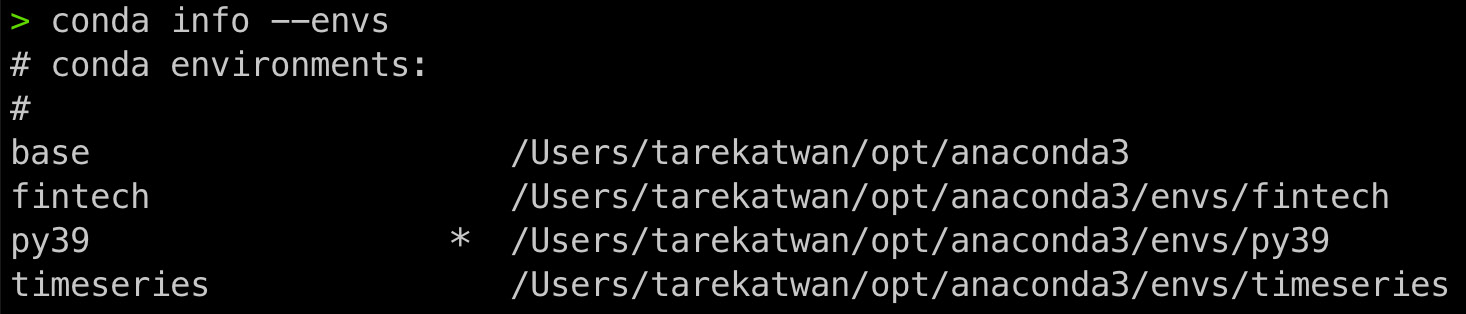
Figure 1.3 – List of all Python virtual environments that have been created using conda

9. Once you activate a specific environment, any package you install will only be available in that isolated environment. For example, let's install the pandas library and specify which version to install in the py39 environment. At the time of writing, pandas 1.4.2 is the latest version:

   $ conda install pandas=1.4.2

Notice that conda will prompt you again for confirmation to let you know what additional package will be downloaded and installed. Here, conda is checking for all the dependencies that pandas 1.4.2 needs and is installing them for you. You can also skip this confirmation step by adding the -y or --yes option at the end of the statement.

The message will also point out the environment location where the installation will occur. The following is an example of a prompted message for installing pandas 1.4.2:

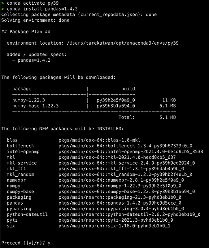
Figure 1.4 – Conda's confirmation prompt listing all the packages

10. Once you press y and hit Enter, conda will begin downloading and installing these packages.
11. Once you are done working in the current py39 environment, you can deactivate and return to the base Python as shown in the following command:

    $ conda deactivate
12. If you no longer need the py39 environment and wish to delete it, you can do so with the env remove command. The command will completely delete the environment and all the installed libraries. In other words, it will delete (remove) the entire folder for that environment:

    $ conda env remove -n py39

Using venv

Once Python 3x has been installed, you get access to the built-in venv module, which allows you to create virtual environments (similar to conda). Notice that when using venv, you will need to provide a path to where you want the virtual environment (folder) to be created. If one isn't provided, it will be created in the current directory where you are running the command from. In the following code, we will create the virtual environment in the Desktop directory.

Follow these steps to create a new environment, install a package, and then delete the environment using venv:

1. First, decide where you want to place the new virtual environment and specify the path. In this example, I have navigated to Desktop and ran the following command:

   $ cd Desktop

   $ python -m venv py3

The preceding code will create a new py3 folder in the Desktop directory. The py3 folder contains several subdirectories, the Python interpreter, standard libraries, and other supporting files. The folder structure is similar to how conda creates its environment folders in the envs directory.

2. Let's activate the py3 environment and examine the $PATH environment variable to verify that it is active. The following script is for Linux and macOS (bash or zsh) and assumes you are running the command from the Desktop directory:

   $ source py3/bin/activate

   $ echo $ PATH

   > /Users/tarekatwan/Desktop/py3/bin:/Users/tarekatwan/opt/anaconda3/bin:/Users/tarekatwan/opt/anaconda3/condabin:/usr/local/bin:/usr/bin:/bin:/usr/sbin:/sbin

Here, we can see that the py3 environment has been activated.

On Windows, there is no bin subfolder, so you will need to run the command using the following syntax, again assuming you are running the command from the Desktop directory:

$ py3/Scripts/activate.bat

If you are running the command in PowerShell, you will need to specify Activate.ps1, as shown in the following:

py3ScriptsActivate.ps1

3. Now, let's check which version has been installed by using the following command:

   $ python --version

   > Python 3.9.12
4. Once you are done developing using the py3 environment, you can deactivate it to return to the base Python environment using the deactivate command:

   $ deactivate
5. If you no longer need the py3 environment and wish to remove it, just delete the entire py3 folder and that's it.

How it works…

Once a virtual environment is activated, you can validate the location of the active Python interpreter to confirm that you are using the right one. Earlier, you saw how the $PATH environment variable changes once you activate a virtual environment. You can achieve similar results using the which command in Linux and macOS, the Get-Command in Windows PowerShell, or the where command in Windows Command Prompt.

The following is an example on macOS:

$ which python
> /Users/tarekatwan/opt/anaconda3/envs/py39/bin/python

This will show the path to the Python interpreter. The output of the preceding statement will show a different path, depending on whether the environment was created with conda or venv. When activating a conda virtual environment, it will be inside the envs folder, as shown in the following:

/Users/tarekatwan/opt/anaconda3/envs/py39/bin/python

When activating a venv virtual environment, the path will be the same path that you provided when it was created, as shown here:

/Users/tarekatwan/Desktop/py3/bin/python

Any additional packages or libraries that you install after you have activated a virtual environment will be isolated from other environments and reside in the environment's folder structure.

If we compare the folder structures of both venv and conda, you can see similarities, as shown in the following screenshot:

Figure 1.5 – Comparing folder structures using conda and venv

Recall that when using conda, all environments will default to the /envs/ location inside the anaconda3/ directory. When using venv, you need to provide a path to specify where to create the directory or project; otherwise, it will default to the current directory that you used to run the command. Similarly, you can specify a different path using conda with the option -p or --prefix. Note that when using venv, you cannot specify the Python version since it relies on the active or base Python version being used to run the command. This is in contrast to conda, which allows you to specify a different Python version regardless of the base Python version installed. For example, the current Python version for the base environment is 3.9.12, and you can create a 3.10.4 environment using the following:

conda create -n py310 python=3.10 -y

The preceding code will create a new py310 environment with Python 3.10.4.

Another advantage of conda, is that it provides two features: a package and dependency manager and a virtual environment manager. This means we can use the same conda environment to create additional environments using conda create, and also install packages using conda install <package name>, which you will use in the next recipe, Installing Python libraries.

Keep in mind that when using venv, it is only a virtual environment manager, and you will still need to rely on pip as a package manager to install packages; for example, pip install <package name>.

Additionally, when using conda to install packages, it will check for any conflicts and will prompt you for any recommendations, including the need to upgrade, downgrade, or install additional package dependencies.

Lastly, an added benefit of using conda is that you can create environments for other languages and not just Python. This includes Julia, R, Lua, Scala, Java, and more.

There's more…

In the preceding examples, you were able to create Python virtual environments from scratch using conda. The virtual environments you created do not contain any packages yet, so you will need to install the required packages for your project.

There are other ways to create your virtual environment in conda that we will discuss here.

Creating a virtual environment using a YAML file

You can create a virtual environment from a YAML file. This option gives greater control in defining many aspects of the environment, including all the packages that should be installed all in one step.

You can create a YAML file in VSCode. Here is an example of a YAML file (env.yml) that creates a conda environment labeled tscookbook using Python 3.9:

#env.yml
name: tscookbook
channels:
  - conda-forge
  - defaults
dependencies:
  - python=3.9
  - pip
  # Data Analysis
  - statsmodels
  - scipy
  - pandas
  - numpy
  - tqdm
  # Plotting
  - matplotlib
  - seaborn
  # Machine learning
  - scikit-learn
  # Jupyter Environment
  - jupyter

To create your virtual environment using the env.yml file, you can use conda env create -f, like so:

$ conda env create -f env.yml

Once this process is completed, you can activate the environment:

$ conda activate tscookbook

You can also bootstrap your YAML file from an existing environment. This is very useful if you want to share your environment configurations with others or create a backup for later use. This can be done with the following command from the activated environment:

$ conda env export > environment.yml

This will generate the environment.yml file for you.

Cloning a virtual environment from another environment

This is a great feature if you want to experiment with new packages or upgrade existing packages, but you do not want to risk breaking the existing code in your current project. Here, you can opt to create a copy of your environment so that you can do your experiments there before you decide whether to proceed with the changes. Cloning can be done in conda with the following command:

$ conda create --name newpy39 --clone py39

See also

It is worth mentioning that Anaconda comes with another tool called anaconda-project to package your conda project artifacts and create a YAML file for reproducibility. Think of this as an alternative approach to developing your YAML manually. For more information, please reference the official GitHub repository here: https://github.com/Anaconda-Platform/anaconda-project.

For a list of arguments, you can type the following in your terminal:

$ anaconda-project --help

If you are using a machine that does not allow you to install any software or you are using an older machine with limited capacity or performance, then do not worry. There are other options so that you can follow the recipes in this book.

Some alternative options that you can explore are as follows:

• Google Colab comprises hosted Python notebooks that already have some of the most popular data science packages preinstalled, including pandas, statsmodels, scikit-learn, and TensorFlow. Colab allows you to install additional packages from within the notebook using pip install. A great feature of Colab is that you get the option to configure your notebook so that you can use a CPU, GPU, or TPU for free. You can explore Colab by going to https://colab.research.google.com/.
• Kaggle Notebooks, similar to Colab, comprises hosted Jupyter notebooks with many of the most popular data science packages already preinstalled. It also allows you to pip install any additional packages that are required. For more information, please refer to https://www.kaggle.com/docs/notebooks.
• Replit offers a free, in-browser IDE that supports more than 50+ languages, including Python. All you need to do is create an account and create your new replit space (https://replit.com/).

Installing Python libraries

In the preceding recipe, you were introduced to the YAML environment configuration file, which allows you to create a Python virtual environment and all the necessary packages in one step using one line of code:

$ conda env create -f environment.yml

Throughout this book, you will need to install several Python libraries to follow the recipes. There are several methods for installing Python libraries, which you will explore in this recipe.

Getting ready

You will create and use different files in this recipe, including a requirements.txt, environment_history.yml, and other files. These files are available to download from the GitHub repository for this book: https://github.com/PacktPublishing/Time-Series-Analysis-with-Python-Cookbook./tree/main/code/Ch1.

In this chapter, you will become familiar with how to generate your requirements.txt file, as well as installing libraries in general.

How to do it…

The easiest way to install a collection of libraries at once is by using a requirements.txt file.

In a nutshell, the requirements.txt file lists the Python libraries and their associated versions that you want to install. You can create your requirements.txt file manually or export it from an existing Python environment.

Using conda

With conda, you have different options for installing our packages in bulk. You can either create a new environment and install all the packages listed in a requirements.txt file at once (using the conda create statement), or you can install the Python packages to an existing environment using the requirements.txt file (using the conda install statement):

• Option 1: Create a new conda environment and install the libraries in one step. For example, you can create a new environment for each chapter and use the associated requirements.txt file:

  $ conda create --name ch1 -f requirements.txt
• Option 2: Install the necessary libraries to an existing conda environment. In this example, you have an existing timeseries environment, which you will need to activate first and then install the libraries from the requirements.txt file:

  $ conda activate timeseries

  $ conda install -f requirements.txt

Using venv and pip

Since venv is just an environment manager, you will need to use pip as your package manager tool. You will start by using venv to create a new environment, and then use pip to install the packages:

• On Mac/Linux: Create and then activate the venv environment before you install the packages:

  $ python -m venv Desktopn/timeseries

  $ source Desktopn/timeseries/bin/activate

  $ pip install -r requirements.txt
• On Windows: Create and activate the venv environment and then install the packages:

  $ python -m venv .Desktop	imeseries

  $ .Desktop	imeseriesScriptsactivate

  $ pip install -r requirements.txt

Notice that in the preceding code for Windows, the activate file extension was not specified (either .bat or .ps1). This is valid and will work on either Windows Prompt or PowerShell.

How it works…

In the preceding code, the requirements.txt file was provided so that you can install the necessary libraries.

But how can you generate your requirements.txt file?

There are two approaches to creating the requirements.txt file. Let's take a look at both.

Creating the file manually

Since it is a simple file format, you can create the file using any text editor, such as VSCode, and list the packages you want to install. If you do not specify the package version, then the latest version that's available will be considered for installation. See the following example for the simple.txt file (hint: the file does not need to be named requirements.txt):

pandas==1.4.2
matplotlib

First, let's test out venv and pip. Run the following script (I am running this on a Mac):

$ python -m venv ch1 
$ source ch1/bin/activate
$ pip install -r simple.txt
$ pip list
Package         Version
--------------- -------
cycler          0.11.0
fonttools       4.33.3
kiwisolver      1.4.2
matplotlib      3.5.2
numpy           1.22.4
packaging       21.3
pandas          1.4.2
Pillow          9.1.1
pip             22.0.4
pyparsing       3.0.9
python-dateutil 2.8.2
pytz            2022.1
setuptools      58.1.0
six             1.16.0
$ deactivate

What are those additional packages? These are based on the dependencies in pandas and matplotlib that pip identified and installed for us.

Now, let's use the same simple.txt file but using conda this time:

$ conda create -n ch1  --file simple.txt python=3.9

Once the installation is completed, you can activate the environment and list the packages that were installed:

$ conda activate ch1
$ conda list 

You may notice that the list is pretty large. More packages are installed compared to the pip approach. You can get a count of the libraries that have been installed using the following command:

$ conda list | wc -l
> 54

There are a few things to keep in mind here:

• conda installs packages from the Anaconda repository, as well as from the Anaconda cloud.
• pip installs packages from Python Package Index (PyPI) repository.
• conda does a very thorough analysis of all the packages it plans to download and does a better job when it comes to version conflicts than pip.

Bootstrapping a file

The second option is to generate the requirements.txt file from an existing environment. This is very useful when you are recreating environments for future use or when sharing your list of packages and dependencies with others, to ensure reproducibility and consistency. Say you worked on a project and installed specific libraries and you want to ensure that when you share your code, other users can install the same libraries. This is where generating the requirements.txt file comes in handy. Similarly, the option to export the YAML environment configuration file was demonstrated earlier.

Let's see how this can be done in both pip and conda. Keep in mind that both methods will export the list of packages that are already installed and their current versions.

venv and pip freeze

pip freeze allows you to export all pip-installed libraries in your environment. First, activate the ch1 environment you created earlier with venv, then export the list of packages to a requirements.txt file. The following example is on a macOS using the Terminal:

$ source ch1/bin/activate
$ pip freeze > requirements.txt
$ cat requirements.txt
>>>
cycler==0.11.0
fonttools==4.33.3
kiwisolver==1.4.2
matplotlib==3.5.2
numpy==1.22.4
...

Once done, you can run the deactivate command.

Conda

Let's activate the environment we created earlier with conda (the ch1 environment) and export the list of packages:

$ conda activate ch1
$ conda list -e > conda_requirements.txt
$ cat conda_requirements.txt
>>>
# This file may be used to create an environment using:
# $ conda create --name <env> --file <this file>
# platform: osx-64
blas=1.0=mkl
bottleneck=1.3.4=py39h67323c0_0
brotli=1.0.9=hb1e8313_2
ca-certificates=2022.4.26=hecd8cb5_0
certifi=2022.5.18.1=py39hecd8cb5_0
cycler=0.11.0=pyhd3eb1b0_0
...

There's more…

When you exported the list of packages installed with conda, the conda_requirements.txt file contained a large list of packages. If you want to export only the packages that you explicitly installed (without the additional packages that conda added), then you can use conda env export command with the --from-history flag:

$ conda activate ch1
$ conda env export --from-history > env.yml
$ cat env.yml
>>>
name: ch1
channels:
  - defaults
dependencies:
  - matplotlib
  - pandas==1.2.0
prefix: /Users/tarek.atwan/opt/anaconda3/envs/ch1

Note that you do not have to activate that environment first, as we have been doing so far. Instead, you can add the -n or --name option to specify the name of the environment. Otherwise, it will default to the currently active environment. This is what the modified script would look like:

conda env export -n ch1 --from-history > env.yml

See also

• To find a list of all the available packages from Anaconda, you can visit https://docs.anaconda.com/anaconda/packages/pkg-docs/.
• To search for package in the PyPI repository, you can visit https://pypi.org/.

Installing JupyterLab and JupyterLab extensions

Throughout this book, you can follow along using your favorite Python IDE (for example, PyCharm or Spyder) or text editor (for example, Visual Studio Code, Atom, or Sublime). There is another option based on the concept of notebooks that allows interactive learning through a web interface. More specifically, Jupyter Notebook or JupyterLab are the preferred methods for learning, experimenting, and following along with the recipes in this book. Interestingly, the name Jupyter is derived from the three programming languages: Julia, Python, and R. Alternatively, you can use Google's Colab or Kaggle Notebooks. For more information, refer to the See also section from the Development environment setup recipe of this chapter. If you are not familiar with Jupyter Notebooks, you can get more information here: https://jupyter.org/.

In this recipe, you will install Jupyter Notebook, JupyterLab, and additional JupyterLab extensions.

Additionally, you will learn how to install individual packages as opposed to the bulk approach we tackled in earlier recipes.

Using Conda in Future Examples

Moving forward, when a new environment is created, the code will be written using conda. The previous recipes already covered the two different approaches to creating virtual environments (venv versus conda) and installing packages (pip versus conda), which should allow you to proceed with whichever choice you prefer.

Getting ready

We will create a new environment and install the main packages needed for this chapter, primarily pandas:

$ conda create -n timeseries python=3.9 pandas -y

This code creates a new Python 3.9 environment named timeseries. The last portion of the statement lists the individual packages that you will be installing. If the list of packages is large, you should use a requirements.txt file instead. If there is a handful of packages, then they can be listed individually separated by spaces, as follows:

$ conda create -n timeseries python=3.9 pandas matplotlib statsmodels -y

Once the environment has been created and the packages have been installed, go ahead and activate it:

$ conda activate timeseries

How to do it…

Now that we have created our environment and activated it, let's install Jupyter:

1. Now that we have activated our environment, we can simply use conda install to install any additional packages that were not included in conda create:

   $ conda install jupyter -y
2. You can launch your JupyterLab instance by typing the following command:

   $ jupyter lab

Notice that this runs a local web server and launches the JupyterLab interface on your default browser, pointing to localhost:8888/lab. The following screenshot shows a similar screen that you would see in your terminal once you've typed in the preceding code:

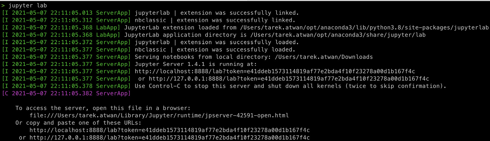
Figure 1.6 – Launching JupyterLab will run a local web server

3. To terminate the web server, press Ctrl + C twice on your terminal or click Shut Down from the File menu in the Jupyter GUI, as shown in the following screenshot:

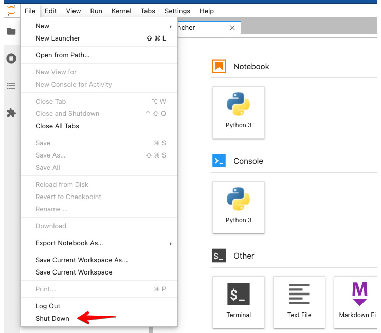
Figure 1.7 – Shutting down the JupyterLab web server

4. Now, you can safely close your browser.
5. Notice that in the preceding example, when JupyterLab was initiated, it launched on your default browser. If you wish to use a different browser, you can update the code like so:

   $ jupyter lab --browser=chrome

In this example, I am specifying that I want it to launch on Chrome as opposed to Safari, which is the default on my machine. You can change the value to your preferred browser, such as Firefox, Opera, Chrome, and so on.

In Windows OS, if the preceding code did not launch Chrome automatically, you will need to register the browser type using webbrowser.register(). To do so, first generate the Jupyter Lab configuration file using the following command:

jupyter-lab --generate-config

Open the jupyter_lab_config.py file and add the following on the top:

import webbrowser 
webbrowser.register('chrome', None, webbrowser.GenericBrowser('C:Program Files (x86)GoogleChromeApplicationchrome.exe'))

Save and close the file. You can rerun jupyter lab --browser=chrome and this should launch the Chrome browser.

6. If you do not want the system to launch the browser automatically, you can do this with the following code:

   $ jupyter lab --no-browser

The web server will start, and you can open any of your preferred browsers manually and just point it to http://localhost:8888.

If you are asked for a token, you can copy and paste the URL with the token as displayed in the Terminal, which looks like this:

To access the server, open this file in a browser:
        file:///Users/tarek.atwan/Library/Jupyter/runtime/jpserver-44086-open.html
    Or copy and paste one of these URLs:
        http://localhost:8888/lab?token=5c3857b9612aecd3
c34e9a40e5eac4509a6ccdbc8a765576
     or http://127.0.0.1:8888/lab?token=5c3857b9612aecd3
c34e9a40e5eac4509a6ccdbc8a765576

7. Lastly, if the default port 8888 is in use or you wish to change the port, then you can add -p and specify the port number you desire, as shown in the following example. Here, I am instructing the web server to use port 8890:

   $ jupyter lab --browser=chrome --port 8890

This will launch Chrome at localhost:8890/lab.

8. Notice that when JupyterLab launches, you only see one kernel in the Notebooks/Console sections. This is the base Python kernel. The expectation was to see two kernels reflecting the two environments we have: the base and the timeseries virtual environment. Let's check how many virtual environments we have with this command:
   1. The following screenshot shows the JupyterLab interface, with only one kernel. This belongs to the base environment:
      

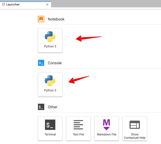
Figure 1.8 – JupyterLab interface showing only one kernel, which belongs to the base environment

2. The following screenshot shows the two Python environments:
   

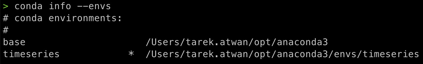
Figure 1.9 – Showing two Python environments

We can see that the timeseries virtual environment is the active one.

9. You will need to install a Jupyter kernel for the new timeseries environment. First, shut down the web server (though it will still work even if you did not). Assuming you are still in the active timeseries Python environment, just type the following command:

   $ python -m ipykernel install --user  --name timeseries --display-name "Time Series"

   > Installed kernelspec timeseries in /Users/tarek.atwan/Library/Jupyter/kernels/timeseries
10. We can check the number of kernels available for Jupyter using the following command:

    $ jupyter kernelspec list

The following screenshot shows the kernelspec files that were created and their location:

Figure 1.10 – List of kernels available for Jupyter

These act as pointers that connect the GUI to the appropriate environment to execute our Python code.

11. Now, you can launch your JupyterLab again and notice the changes:

    $ jupyter lab

The following screen will appear once it has been launched:

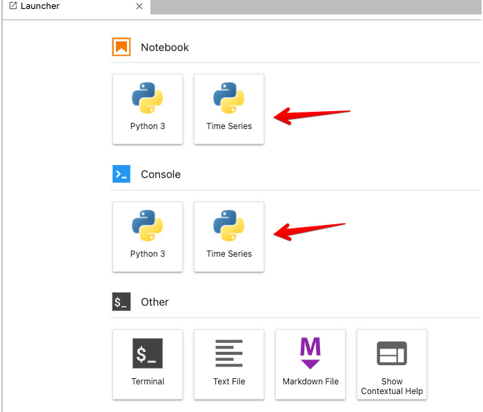
Figure 1.11 – Notice now our Time Series kernel is available in JupyterLab

How it works…

When you created the new timeseries environment and installed our desired packages using conda install, it created a new subfolder inside the envs folder to isolate the environment and packages installed from other environments, including the base environment. When executing the jupyter notebook or jupyter lab command from the base environment, it will need to read from a kernelspec file (JSON) to map to the available kernels in order to make them available. The kernelspec file can be created using ipykernel, like so:

python -m ipykernel install --user  --name timeseries --display-name "Time Series"

Here, --name refers to the environment name and --display-name refers to the display name in the Jupyter GUI, which can be anything you want. Now, any libraries that you install inside the timeseries environment can be accessed from Jupyter through the kernel (again, think of it as a mapping between the Jupyter GUI and the backend Python environment).

There's more…

JupyterLab allows you to install several useful extensions. Some of these extensions are created and managed by Jupyter, while others are created by the community.

You can manage JupyterLab extensions in two ways: through the command line using jupyter labextension install <someExtension> or through the GUI using Extension Manager. The following screenshot shows what the Jupyter Extension Manager UI looks like:

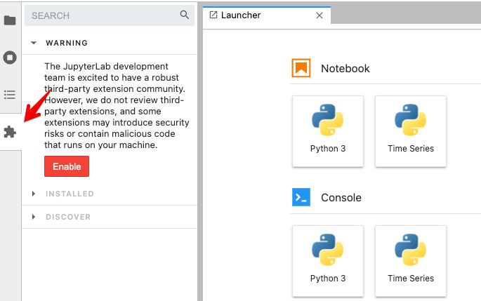
Figure 1.12 – Clicking the extension manager icon in JupyterLab

Once you click Enable, you will see a list of available Jupyter extensions. To install an extension, just click on the Install button.

Some packages will require Node.js and npm to be installed first and you will see a warning similar to the following:

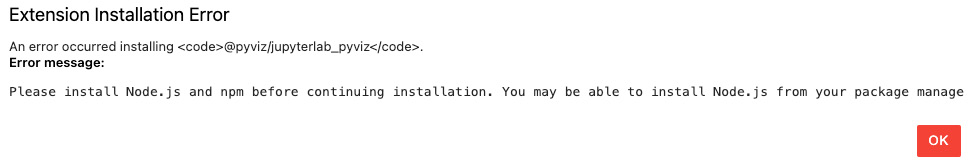
Figure 1.13 – Extension Installation Error when Node.js is required

You can download and install Node.js directly from https://nodejs.org/en/.

Alternatively, you can use conda to install Node.js by using the following command:

$ conda install -c conda-forge nodejs

See also

• To learn more about JupyterLab extensions, please refer to the official documentation here: https://jupyterlab.readthedocs.io/en/stable/user/extensions.html.
• If you want to learn more about how JupyterLab extensions are created with example demos, please refer to the official GitHub repository here: https://github.com/jupyterlab/extension-examples.
• In step 9, we manually installed the kernelspec files, which created the mapping between Jupyter and our conda environment. This process can be automated using nb_conda. For more information on the nb_conda project, please refer to the official GitHub repository here: https://github.com/Anaconda-Platform/nb_conda.