
Outlier Detection Using Unsupervised Machine Learning
In Chapter 8, Outlier Detection Using Statistical Methods, you explored parametric and non-parametric statistical techniques to spot potential outliers. The methods were simple, interpretable, and yet quite effective.
Outlier detection is not straightforward, mainly due to the ambiguity surrounding the definition of what an outlier is specific to your data or the problem that you are trying to solve. For example, though common, some of the thresholds used in Chapter 8, Outlier Detection Using Statistical Methods, are still arbitrary and not a rule that you should follow. Therefore, having domain knowledge is vital to making the proper judgment when spotting outliers.
In this chapter, you will be introduced to a handful of machine learning-based methods for outlier detection. Most of the machine learning techniques for outlier detection are considered unsupervised outlier detection methods, such as Isolation Forests (iForest), unsupervised K-Nearest Neighbors (KNN), Local Outlier Factor (LOF), and Copula-Based Outlier Detection (COPOD), to name a few.
Generally, outliers (or anomalies) are considered a rare occurrence (later in the chapter, you will see this referenced as the contamination percentage). In other words, you would assume a small fraction of your data are outliers in a large data set. For example, 1% of the data may be potential outliers. However, this complexity requires methods designed to find patterns in the data. Unsupervised outlier detection techniques are great at finding patterns in rare occurrences.
After investigating outliers, you will have a historical set of labeled data, allowing you to leverage semi-supervised outlier detection techniques. This chapter focuses on unsupervised outlier detection.
In this chapter, you will be introduced to the PyOD library, described as "a comprehensive and scalable Python toolkit for detecting outlying objects in multivariate data." The library offers an extensive collection of implementations for popular and emerging algorithms in the field of outlier detection, which you can read about here: https://github.com/yzhao062/pyod.
You will be using the same New York taxi dataset to make it easier to compare the results between the different machine learning methods in this chapter and the statistical methods from Chapter 8, Outlier Detection Using Statistical Methods.
The recipes that you will encounter in this chapter are as follows:
- Detecting outliers using KNN
- Detecting outliers using LOF
- Detecting outliers using iForest
- Detecting outliers using One-Class Support Vector Machine (OCSVM)
- Detecting outliers using COPOD
- Detecting outliers with PyCaret
Technical requirements
You can download the Jupyter notebooks and datasets required from the GitHub repository:
- Jupyter notebooks: https://github.com/PacktPublishing/Time-Series-Analysis-with-Python-Cookbook./blob/main/code/Ch14/Chapter%2014.ipynb
- Datasets: https://github.com/PacktPublishing/Time-Series-Analysis-with-Python-Cookbook./tree/main/datasets/Ch14
You can install PyOD with either pip or Conda. For a pip install, run the following command:
pip install pyod
For a Conda install, run the following command:
conda install -c conda-forge pyod
To prepare for the outlier detection recipes, start by loading the libraries that you will be using throughout the chapter:
import pandas as pd
import numpy as np
import matplotlib.pyplot as plt
from pathlib import Path
import warnings
warnings.filterwarnings('ignore')
plt.rcParams["figure.figsize"] = [16, 3]
Load the nyc_taxi.csv data into a pandas DataFrame as it will be used throughout the chapter:
file = Path("../../datasets/Ch8/nyc_taxi.csv")
nyc_taxi = pd.read_csv(folder / file,
                     index_col='timestamp',
                     parse_dates=True)
nyc_taxi.index.freq = '30T'
You can store the known dates containing outliers, also known as ground truth labels:
nyc_dates =  [
        "2014-11-01",
        "2014-11-27",
        "2014-12-25",
        "2015-01-01",
        "2015-01-27"]
Create the plot_outliers function that you will use throughout the recipes:
def plot_outliers(outliers, data, method='KNN',
                 halignment = 'right',
                 valignment = 'top',
                 labels=False):
    ax = data.plot(alpha=0.6)

    if labels:
        for i in outliers['value'].items():
            plt.plot(i[0], i[1], 'v', markersize=8, markerfacecolor='none', markeredgecolor='k')
            plt.text(i[0], i[1]-(i[1]*0.04), f'{i[0].strftime("%m/%d")}',
                         horizontalalignment=halignment,
                         verticalalignment=valignment)
    else:
        data.loc[outliers.index].plot(ax=ax, style='rX', markersize=9)
    plt.title(f'NYC Taxi - {method}')
    plt.xlabel('date'); plt.ylabel('# of passengers')
    plt.legend(['nyc taxi','outliers'])
    plt.show()
As you proceed with the outlier detection recipes, the goal is to see how the different techniques capture outliers and compare them to the ground truth labels, as follows:
tx = nyc_taxi.resample('D').mean()
known_outliers = tx.loc[nyc_dates]
plot_outliers(known_outliers, tx, 'Known Outliers')
The preceding code should produce a time series plot with X markers for the known outliers:
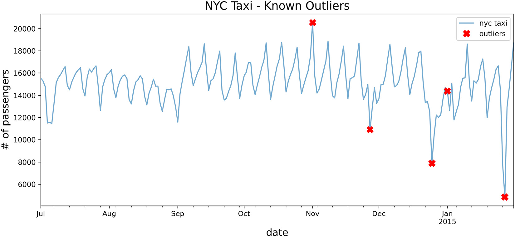
Figure 14.1 – Plotting the NYC taxi data after downsampling with ground truth labels (outliers)
PyOD's Methods for Training and Making Predictions
Like scikit-learn, PyOD offers familiar methods for training your model and making predictions by providing three methods: model.fit(), model.predict(), and model.fit_predict().
In the recipes, we will break down the process into two steps by first fitting the model (training) using .fit() and then making a prediction using .predict().
In addition to the predict method, PyOD provides two additional methods: predict_proba and predict_confidence.
In the first recipe, you will explore how PyOD works behind the scenes and introduce fundamental concepts, for example, the concept of contamination and how threshold_ and decision_scores_ are used to generate the binary labels (abnormal or normal). These concepts will be covered in more depth in the following recipe.
Detecting outliers using KNN
The KNN algorithm is typically used in a supervised learning setting where prior results or outcomes (labels) are known.
It can be used to solve classification or regression problems. The idea is simple; for example, you can classify a new data point, Y, based on its nearest neighbors. For instance, if k=5, the algorithm will find the five nearest data points (neighbors) by distance to the point Y and determine its class based on the majority. If there are three blue and two red nearest neighbors, Y is classified as blue. The K in KNN is a parameter you can modify to find the optimal value.
In the case of outlier detection, the algorithm is used differently. Since we do not know the outliers (labels) in advance, KNN is used in an unsupervised learning manner. In this scenario, the algorithm finds the closest K nearest neighbors for every data point and measures the average distance. The points with the most significant distance from the population will be considered outliers, and more specifically, they are considered global outliers. In this case, the distance becomes the score to determine which points are outliers among the population, and hence KNN is a proximity-based algorithm.
Generally, proximity-based algorithms rely on the distance or proximity between an outlier point and its nearest neighbors. In KNN, the number of nearest neighbors, k, is a parameter you need to determine. There are other variants of the KNN algorithm supported by PyOD, for example, Average KNN (AvgKNN), which uses the average distance to the KNN for scoring, and Median KNN (MedKNN), which uses the median distance for scoring.
How to do it...
In this recipe, you will continue to work with the tx DataFrame, created in the Technical requirements section, to detect outliers using the KNN class from PyOD:
- Start by loading the KNN class:
from pyod.models.knn import KNN
- You should be familiar with a few parameters to control the algorithm's behavior. The first parameter is contamination, a numeric (float) value representing the dataset's fraction of outliers. This is a common parameter across all the different classes (algorithms) in PyOD. For example, a contamination value of 0.1 indicates that you expect 10% of the data to be outliers. The default value is contamination=0.1. The contamination value can range from 0 to 0.5 (or 50%). You will need to experiment with the contamination value, since the value influences the scoring threshold used to determine potential outliers, and how many of these potential outliers are to be returned. You will learn more about this in the How it works... section of this chapter.
For example, if you suspect the proportion of outliers in your data at 3%, then you can use that as the contamination value. You could experiment with different contamination values, inspect the results, and determine how to adjust the contamination level. We already know that there are 5 known outliers out of the 215 observations (around 2.3%), and in this recipe, you will use 0.03 (or 3%).
The second parameter, specific to KNN, is method, which defaults to method='largest'. In this recipe, you will change it to the mean (the average of all k neighbor distances). The third parameter, also specific to KNN, is metric, which tells the algorithm how to compute the distances. The default is the minkowski distance but it can take any distance metrics from scikit-learn or the SciPy library. Finally, you need to provide the number of neighbors, which defaults to n_neighbors=5. Ideally, you will want to run for different KNN models with varying values of k and compare the results to determine the optimal number of neighbors.
- Instantiate KNN with the updated parameters and then train (fit) the model:
knn = KNN(contamination=0.03,
method='mean',
n_neighbors=5)
knn.fit(tx)
>>
KNN(algorithm='auto', contamination=0.05, leaf_size=30, method='mean',
metric='minkowski', metric_params=None, n_jobs=1, n_neighbors=5, p=2,
radius=1.0)
- The predict method will generate binary labels, either 1 or 0, for each data point. A value of 1 indicates an outlier. Store the results in a pandas Series:
predicted = pd.Series(knn.predict(tx),
index=tx.index)
print('Number of outliers = ', predicted.sum())>>
Number of outliers = 6
- Filter the predicted Series to only show the outlier values:
outliers = predicted[predicted == 1]
outliers = tx.loc[outliers.index]
outliers
>>
Timestamp value
2014-11-01 20553.500000
2014-11-27 10899.666667
2014-12-25 7902.125000
2014-12-26 10397.958333
2015-01-26 7818.979167
2015-01-27 4834.541667
Overall, the results look promising; four out of the five known dates have been identified. Additionally, the algorithm identified the day after Christmas as well as January 26, 2015, which was when all vehicles were ordered off the street due to the North American blizzard.
- Use the plot_outliers function created in the Technical requirements section to visualize the output to gain better insight:
plot_outliers(outliers, tx, 'KNN')
The preceding code should produce a plot similar to that in Figure 14.1, except the x markers are based on the outliers identified using the KNN algorithm:
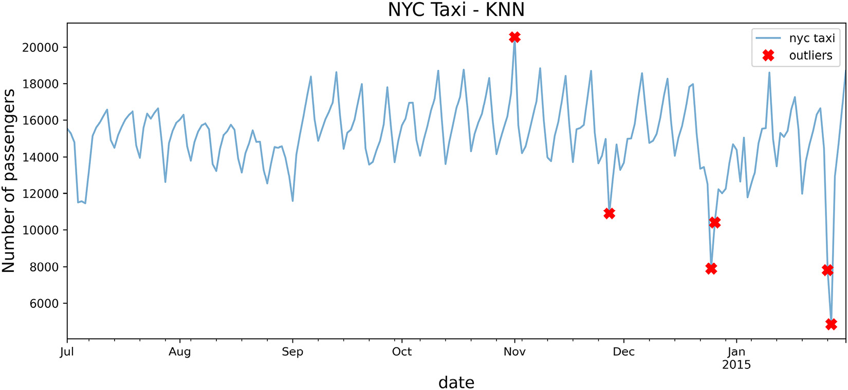
Figure 14.2 – Markers showing the identified potential outliers using the KNN algorithm
To print the labels (dates) along with the markers, just call the plot_outliers function again, but this time with labels=True:
plot_outliers(outliers, tx, 'KNN', labels=True)
The preceding code should produce a similar plot to the one in Figure 14.2 with the addition of text labels.
How it works...
The unsupervised approach to the KNN algorithm calculates the distance of an observation to other neighboring observations. The default distance used in PyOD for KNN is the Minkowski distance (the p-norm distance). You can change to different distance measures, such as the Euclidean distance with euclidean or l2 or the Manhattan distance with manhattan or l1. This can be accomplished using the metric parameter, which can take a string value, for example, metric='l2' or metric='euclidean', or a callable function from scikit-learn or SciPy. This is a parameter that you experiment with as it influences how the distance is calculated, which is what the outlier scores are based on.
Traditionally, when people hear KNN, they immediately assume it is only a supervised learning algorithm. For unsupervised KNN, there are three popular algorithms: ball tree, KD tree, and brute-force search. The PyOD library supports all three as ball_tree, kd_tree, and brute, respectively. The default value is set to algorithm="auto".
PyOD uses an internal score specific to each algorithm, scoring each observation in the training set. The decision_scores_ attribute will show these scores for each observation. Higher scores indicate a higher potential of being an abnormal observation:
knn_scores = knn.decision_scores_
You can convert this into a DataFrame:
knn_scores_df = (pd.DataFrame(scores,
             index=tx.index,
             columns=['score']))
knn_scores_df
Since all the data points are scored, PyOD will determine a threshold to limit the number of outliers returned. The threshold value depends on the contamination value you provided earlier (the proportion of outliers you suspect). The higher the contamination value, the lower the threshold, and hence more outliers are returned. A lower contamination value will increase the threshold.
You can get the threshold value using the threshold_ attribute from the model after fitting it to the training data. Here is the threshold for KNN based on a 3% contamination rate:
knn.threshold_
>> 225.0179166666657
This is the value used to filter out the significant outliers. Here is an example of how you reproduce that:
knn_scores_df[knn_scores_df['score'] >= knn.threshold_].sort_values('score', ascending=False)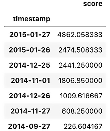
Figure 14.3 – Showing the decision scores from PyOD
Notice the last observation on 2014-09-27 is slightly above the threshold, but it was not returned when you used the predict method. If you use the contamination threshold, you can get a better cutoff:
n = int(len(tx)*0.03)
knn_scores_df.nlargest(n, 'score')
Another helpful method is predict_proba, which returns the probability of being normal and the probability of being abnormal for each observation. PyOD provides two methods for determining these percentages: linear or unify. The two methods scale the outlier scores before calculating the probabilities. For example, in the case of linear, the implementation uses MinMaxScaler from scikit-learn to scale the scores before calculating the probabilities. The unify method uses the z-score (standardization) and the Gaussian error function (erf) from the SciPy library (scipy.special.erf).
You can compare the two approaches. First, start using the linear method to calculate the prediction probability, you can use the following:
knn_proba = knn.predict_proba(tx, method='linear')
knn_proba_df = (pd.DataFrame(np.round(knn_proba * 100, 3),
            index=tx.index,
            columns=['Proba_Normal', 'Proba_Anomaly']))
knn_proba_df.nlargest(n, 'Proba_Anomaly')
For the unify method, you can just update method='unify'.
To save any PyOD model, you can use the joblib Python library:
from joblib import dump, load
# save the knn model
dump(knn, 'knn_outliers.joblib')
# load the knn model
knn = load('knn_outliers.joblib')
There's more...
Earlier in the recipe, when instantiating the KNN class, you changed the value of method for calculating the outlier score to be mean:
knn = KNN(contamination=0.03,
          method='mean',
          n_neighbors=5)
Let's create a function for the KNN algorithm to train the model on different scoring methods by updating the method parameter to either mean, median, or largest to examine the impact on the decision scores:
- largest uses the largest distance to the kth neighbor as the outlier score.
- mean uses the average of the distances to the k neighbors as the outlier score.
- median uses the median of the distances to the k neighbors as the outlier score.
Create the knn_anomaly function with the following parameters: data, method, contamination, and k:
def knn_anomaly(df, method='mean', contamination=0.05, k=5):
    knn = KNN(contamination=contamination,
              method=method,
              n_neighbors=5)
    knn.fit(df)
    decision_score = pd.DataFrame(knn.decision_scores_,
                          index=df.index, columns=['score'])
    n = int(len(df)*contamination)
    outliers = decision_score.nlargest(n, 'score')
    return outliers, knn.threshold_
You can run the function using different methods, contamination, and k values to experiment.
Explore how the different methods produce a different threshold, which impacts the outliers being detected:
for method in ['mean', 'median', 'largest']:
    o, t = knn_anomaly(tx, method=method)
    print(f'Method= {method}, Threshold= {t}')
    print(o)
The preceding code should print out the top 10 outliers for each method (with contamination at 5%):
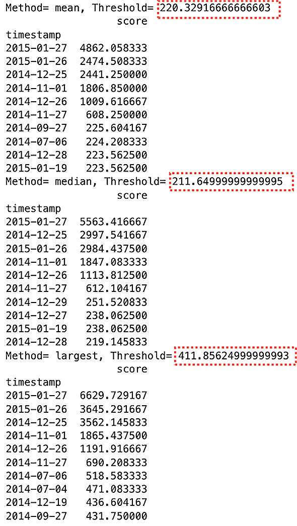
Figure 14.4 – Comparing decision scores using different KNN distance metrics
Notice the top six (represent the 3% contamination) are identical for all three methods. The order may vary and the decision scores are different between the methods. Do notice the difference between the methods is more apparent beyond the top six, as shown in Figure 14.4.
See also
Check out the following resources:
- To learn more about unsupervised KNN, the scikit-learn library has a great explanation about its implementation: https://scikit-learn.org/stable/modules/neighbors.html#unsupervised-nearest-neighbors.
- To learn more about PyOD KNN and the different parameters, visit the official documentation here: https://pyod.readthedocs.io/en/latest/pyod.models.html?highlight=knn#module-pyod.models.knn.
Detecting outliers using LOF
In the previous recipe, Detecting outliers using KNN, in the KNN algorithm, the decision scoring for detecting outliers was based on the distance between observations. A data point far from its KNN can be considered an outlier. Overall, the algorithm does a good job of capturing global outliers, but those far from the surrounding points may not do well with identifying local outliers.
This is where the LOF comes in to solve this limitation. Instead of using the distance between neighboring points, it uses density as a basis for scoring data points and detecting outliers. The LOF is considered a density-based algorithm. The idea behind the LOF is that outliers will be further from other data points and more isolated, and thus will be in low-density regions.
It is easier to illustrate this with an example: imagine a person standing in line in a small but busy Starbucks, and everyone is pretty much close to each other; then, we can say the person is in a high-density area and, more specifically, high local density. If the person decides to wait in their car in the parking lot until the line eases up, they are isolated and in a low-density area, thus being considered an outlier. From the perspective of the people standing in line, who are probably not aware of the person in the car, that person is considered not reachable even though that person in the vehicle can see all of the individuals standing in line. So we say that the person in the car is not reachable from their perspective. Hence, we sometimes refer to this as inverse reachability (how far you are from the neighbors' perspective, not just yours).
Like KNN, you still need to define the k parameter for the number of nearest neighbors. The nearest neighbors are identified based on the distance measured between the observations (think KNN), then the Local Reachability Density (LRD or local density for short) is measured for each neighboring point. This local density is the score used to compare the kth neighboring observations and those with lower local densities than their kth neighbors are considered outliers (they are further from the reach of their neighbors).
How to do it...
In this recipe, you will continue to work with the tx DataFrame, created in the Technical requirements section, to detect outliers using the LOF class from PyOD:
- Start by loading the LOF class:
from pyod.models.lof import LOF
- You should be familiar with a few parameters to control the algorithm's behavior. The first parameter is contamination, a numeric (float) value representing the dataset's fraction of outliers. For example, a value of 0.1 indicates that you expect 10% of the data to be outliers. The default value is contamination=0.1. In this recipe, you will use 0.03 (3%).
The second parameter is the number of neighbors, which defaults to n_neighbors=5, similar to the KNN algorithm. Ideally, you will want to run different models with varying values of k (n_neighbors) and compare the results to determine the optimal number of neighbors. Lastly, the metric parameter specifies which metric to use to calculate the distance. This can be any distance metrics from the scikit-learn or SciPy libraries (for example, Euclidean or Manhattan distance). The default value is the Minkowski distance with metric='minkowski'. Since the Minkowski distance is a generalization for both the Euclidean (![]() ) and Manhattan distances (
) and Manhattan distances (![]() ), you will notice a p parameter. By default, p=2 indicates Euclidean distance, while a value of p=1 indicates Manhattan distance.
), you will notice a p parameter. By default, p=2 indicates Euclidean distance, while a value of p=1 indicates Manhattan distance.
- Instantiate LOF by updating n_neighbors=5 and contamination=0.03 while keeping the rest of the parameters with the default values. Then, train (fit) the model:
lof = LOF(contamination=0.03, n_neighbors=5)
lof.fit(tx)
>>
LOF(algorithm='auto', contamination=0.03, leaf_size=30, metric='minkowski',
metric_params=None, n_jobs=1, n_neighbors=5, novelty=True, p=2)
- The predict method will output either 1 or 0 for each data point. A value of 1 indicates an outlier. Store the results in a pandas Series:
predicted = pd.Series(lof.predict(tx),
index=tx.index)
print('Number of outliers = ', predicted.sum())>>
Number of outliers = 6
- Filter the predicted Series to only show the outlier values:
outliers = predicted[predicted == 1]
outliers = tx.loc[outliers.index]
outliers
>>
Timestamp value
2014-10-31 17473.354167
2014-11-01 20553.500000
2014-12-25 7902.125000
2014-12-26 10397.958333
2015-01-26 7818.979167
2015-01-27 4834.541667
Interestingly, it captured three out of the five known dates but managed to identify the day after Thanksgiving and the day after Christmas as outliers. Additionally, October 31 was on a Friday, and it was Halloween night.
- Use the plot_outliers function created in the Technical requirements section to visualize the output to gain better insight:
plot_outliers(outliers, tx, 'LOF')
The preceding code should produce a plot similar to that in Figure 14.1, except the x markers are based on the outliers identified using the LOF algorithm:
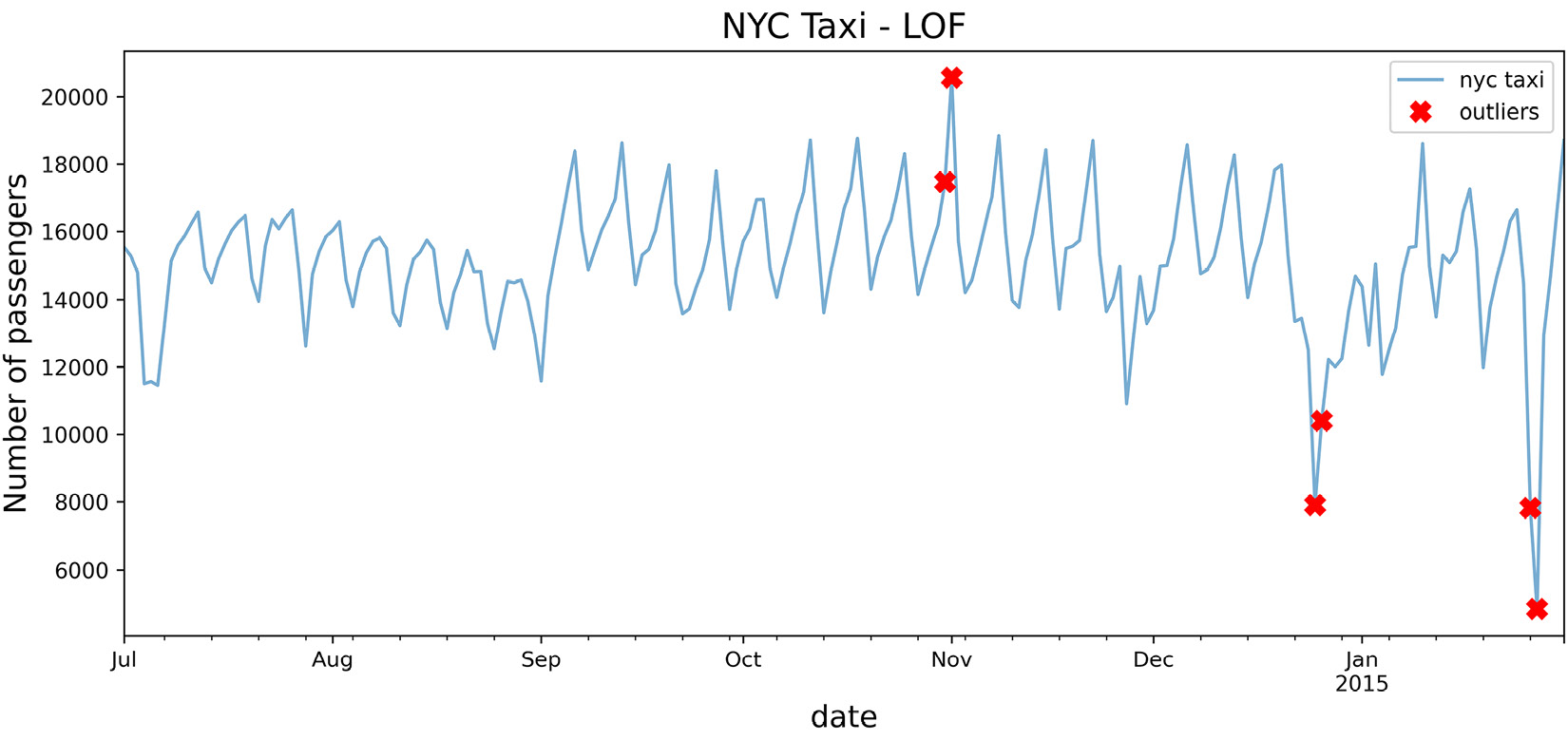
Figure 14.5 – Markers showing the identified potential outliers using the LOF algorithm
To print the labels (dates) with the markers, just call the plot_outliers function again but this time with labels=True:
plot_outliers(outliers, tx, 'LOF', labels=True)
The preceding code should produce a similar plot to the one in Figure 14.5 with the addition of text labels.
How it works...
The LOF is a density-based algorithm that assumes that outlier points are more isolated and have lower local density scores compared to their neighbors.
LOF is like KNN in that we measure the distances between the neighbors before calculating the local density. The local density is the basis of the decision scores, which you can view using the decision_scores_ attribute:
timestamp  score
2014-11-01  14.254309
2015-01-27  5.270860
2015-01-26  3.988552
2014-12-25  3.952827
2014-12-26  2.295987
2014-10-31  2.158571
The scores are very different from those in Figure 14.3 for KNN.
For more insight into decision_scores_, threshold_, or predict_proba, please review the first recipe of this chapter, Detecting outliers using KNN.
There's more...
Like the LOF, another extension of the algorithm is the Cluster-Based Local Outlier Factor (CBLOF). The CBLOF is similar to LOF in concept as it relies on cluster size and distance when calculating the scores to determine outliers. So, instead of the number of neighbors (n_neighbors like in LOF), we now have a new parameter, which is the number of clusters (n_clusters).
The default clustering estimator, clustering_estimator, in PyOD is the k-means clustering algorithm.
You will use the CBLOF class from PyOD and keep most parameters at the default values. Change the n_clusters=8 and contamination=0.03 parameters:
from pyod.models.cblof import CBLOF
cblof = CBLOF(n_clusters=4, contamination=0.03)
cblof.fit(tx)
predicted = pd.Series(lof.predict(tx),
                      index=tx.index)
outliers = predicted[predicted == 1]
outliers = tx.loc[outliers.index]
plot_outliers(outliers, tx, 'CBLOF')
The preceding code should produce a plot similar to that in Figure 14.1 except the x markers are based on the outliers identified using the CBLOF algorithm:
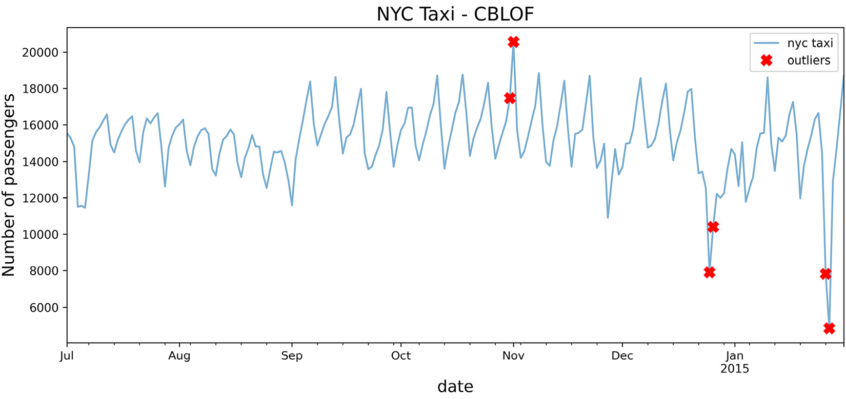
Figure 14.6 – Markers showing the identified potential outliers using the CBLOF algorithm
Compare Figure 14.6 with Figure 14.5 (LOF) and notice the similarity.
See also
To learn more about the LOF and CBLOF algorithms, you can visit the PyOD documentation:
- LOF: https://pyod.readthedocs.io/en/latest/pyod.models.html#module-pyod.models.lof
- CBLOF: https://pyod.readthedocs.io/en/latest/pyod.models.html#module-pyod.models.cblof
Detecting outliers using iForest
iForest has similarities with another popular algorithm known as Random Forests. Random Forests is a tree-based supervised learning algorithm. In supervised learning, you have existing labels (classification) or values (regression) representing the target variable. This is how the algorithm learns (it is supervised).
The name forest stems from the underlying mechanism of how the algorithm works. For example, in classification, the algorithm randomly samples the data to build multiple weak classifiers (smaller decision trees) that collectively make a prediction. In the end, you get a forest of smaller trees (models). This technique outperforms a single complex classifier that may overfit the data. Ensemble learning is the concept of multiple weak learners collaborating to produce an optimal solution.
iForest, also an ensemble learning method, is the unsupervised learning approach to Random Forests. The iForest algorithm isolates anomalies by randomly partitioning (splitting) a dataset into multiple partitions. This is performed recursively until all data points belong to a partition. The number of partitions required to isolate an anomaly is typically smaller than the number of partitions needed to isolate a regular point. The idea is that an anomaly data point is further from other points and thus easier to separate (isolate).
In contrast, a normal data point is probably clustered closer to the larger set and, therefore, will require more partitions (splits) to isolate that point. Hence the name, isolation forest, since it identifies outliers through isolation. Once all the points are isolated, the algorithm will create an outlier score. You can think of these splits as creating a decision tree path. The shorter the path length to a point, the higher the chances of an anomaly.
How to do it...
In this recipe, you will continue to work with the nyc_taxi DataFrame to detect outliers using the IForest class from the PyOD library:
- Start by loading the IForest class:
from pyod.models.iforest import IForest
- There are a few parameters that you should be familiar with to control the algorithm's behavior. The first parameter is contamination. The default value is contamination=0.1 but in this recipe, you will use 0.03 (3%).
The second parameter is n_estimators, which defaults to n_estimators=100. This is the number of random trees generated. Depending on the complexity of your data, you may want to increase this value to a higher range, such as 500 or more. Start with the default smaller value to understand how the baseline model works—finally, random_state defaults to None. Since the iForest algorithm randomly generates partitions for the data, it is good to set a value to ensure that your work is reproducible. This way, you can get consistent results back when you rerun the code. Of course, this could be any integer value.
- Instantiate IForest and update the contamination and random_state parameters. Then, fit the new instance of the class (iforest) on the resampled data to train the model:
iforest = IForest(contamination=0.03,
n_estimators=100,
random_state=0)
iforest.fit(nyc_daily)
>>
IForest(behaviour='old', bootstrap=False, contamination=0.03,
max_features=1.0, max_samples='auto', n_estimators=100, n_jobs=1,
random_state=0, verbose=0)
- Use the predict method to identify outliers. The method will output either 1 or 0 for each data point. For example, a value of 1 indicates an outlier.
Let's store the results in a pandas Series:
predicted = pd.Series(iforest.predict(tx),
                      index=tx.index)
print('Number of outliers = ', predicted.sum())
>>
Number of outliers =  7
Interestingly, unlike the previous recipe, Detecting outliers using KNN, iForest detected 7 outliers while the KNN algorithm detected 6.
- Filter the predicted Series to only show the outlier values:
outliers = predicted[predicted == 1]
outliers = tx.loc[outliers.index]
outliers
>>
timestamp value
2014-11-01 20553.500000
2014-11-08 18857.333333
2014-11-27 10899.666667
2014-12-25 7902.125000
2014-12-26 10397.958333
2015-01-26 7818.979167
2015-01-27 4834.541667
Overall, iForest captured four out of the five known outliers. There are additional but interesting dates identified that should trigger an investigation to determine whether these data points are outliers. For example, November 8, 2014, was detected as a potential outlier by the algorithm, which was not considered in the data.
- Use the plot_outliers function created in the Technical requirements section to visualize the output to gain better insight:
plot_outliers(outliers, tx, 'IForest')
The preceding code should produce a plot similar to that in Figure 14.1 except the x markers are based on the outliers identified using the iForest algorithm:
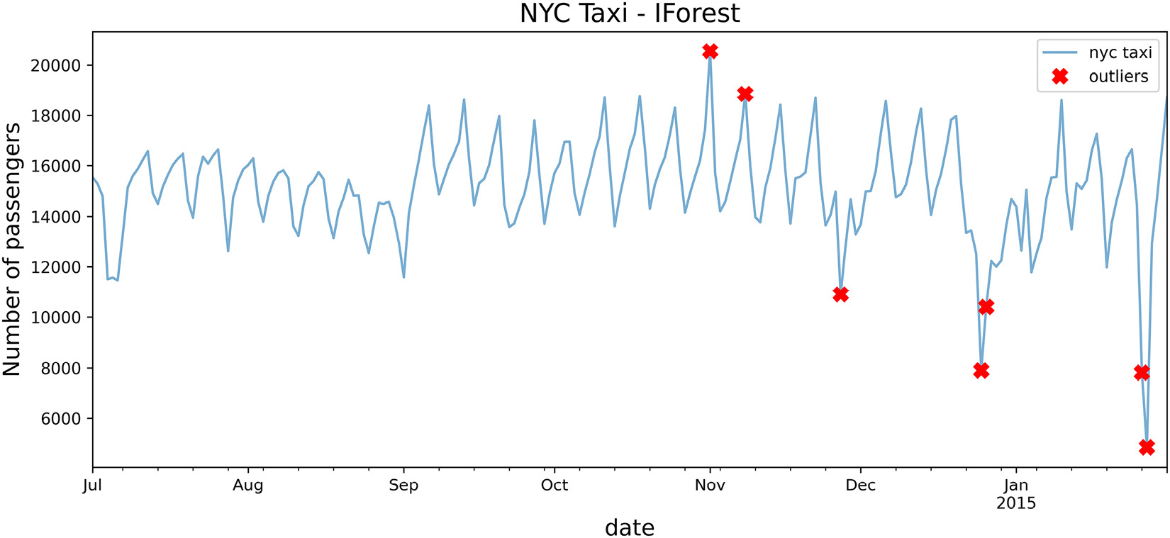
Figure 14.7 – Markers showing the identified potential outliers using the iForest algorithm
To print the labels (dates) with the markers, just call the plot_outliers function again but this time with labels=True:
plot_outliers(outliers, tx, 'IForest', labels=True)
The preceding code should produce a similar plot as the one in Figure 14.7 with the addition of text labels.
How it works...
Since iForest is an ensemble method, you will be creating multiple models (tree learners). The default value of n_estimators is 100. Increasing the number of base estimators may improve model performance up to a certain level before the computational performance takes a hit. So, for example, think of the number of estimators as trained models. For instance, for 100 estimators, you are essentially creating 100 decision tree models.
There is one more parameter worth mentioning, which is the bootstrap parameter. It is a Boolean set to False by default. Since iForest randomly samples the data, you have two options: random sampling with replacement (known as bootstrapping) or random sampling without replacement. The default behavior is sampling without replacement.
There's more...
The iForest algorithm from PyOD (the IForest class) is a wrapper to scikit-learn's IsolationForest class. This is also true for the KNN used in the previous recipe, Detecting outliers using KNN.
Let's explore this further and use scikit-learn to implement the iForest algorithm. You will use the fit_predict() method as a single step to train and predict, which is also available in PyOD's implementations across the various algorithms:
from sklearn.ensemble import IsolationForest
sk_iforest = IsolationForest(contamination=0.03)
sk_prediction = pd.Series(sk_iforest.fit_predict(tx),
                      index=tx.index)
sk_outliers = sk_prediction[sk_prediction == -1]
sk_outliers = tx.loc[sk_outliers.index]
sk_outliers
>>
timestamp   value
2014-11-01  20553.500000
2014-11-08  18857.333333
2014-11-27  10899.666667
2014-12-25  7902.125000
2014-12-26  10397.958333
2015-01-26  7818.979167
2015-01-27  4834.541667
The results are the same. But do notice that, unlike PyOD, the identified outliers were labeled as -1, while in PyOD, outliers were labeled with 1.
See also
The PyOD iForest implementation is actually a wrapper to the IsolationForest class from scikit-learn:
- To learn more about PyOD iForest and the different parameters, visit their official documentation here: https://pyod.readthedocs.io/en/latest/pyod.models.html?highlight=knn#module-pyod.models.iforest.
- To learn more about the IsolationForest class from scikit-learn, you can visit their official documentation page here: https://scikit-learn.org/stable/modules/generated/sklearn.ensemble.IsolationForest.html#sklearn-ensemble-isolationforest.
Detecting outliers using One-Class Support Vector Machine (OCSVM)
Support Vector Machine (SVM) is a popular supervised machine learning algorithm that is mainly known for classification but can also be used for regression. The popularity of SVM comes from the use of kernel functions (sometimes referred to as the kernel trick), such as linear, polynomial, Radius-Based Function (RBF), and the sigmoid function.
In addition to classification and regression, SVM can also be used for outlier detection in an unsupervised manner, similar to KNN, which is mostly known as a supervised machine learning technique but was used in an unsupervised manner for outlier detection, as seen in the Outlier detection using KNN recipe.
How to do it...
In this recipe, you will continue to work with the tx DataFrame, created in the Technical requirements section, to detect outliers using the ocsvm class from PyOD:
- Start by loading the OCSVM class:
from pyod.models.ocsvm import OCSVM
- There are a few parameters that you should be familiar with to control the algorithm's behavior. The first parameter is contamination. The default value is contamination=0.1 and in this recipe, you will use 0.03 (3%).
The second parameter is kernel, which is set to rbf, which you will keep as is.
Instantiate OCSVM by updating contamination=0.03 while keeping the rest of the parameters with the default values. Then, train (fit) the model:
ocsvm = OCSVM(contamination=0.03, kernel='rbf')
ocsvm.fit(tx)
>>
OCSVM(cache_size=200, coef0=0.0, contamination=0.03, degree=3, gamma='auto',
   kernel='rbf', max_iter=-1, nu=0.5, shrinking=True, tol=0.001,
   verbose=False)
- The predict method will output either 1 or 0 for each data point. A value of 1 indicates an outlier. Store the results in a pandas Series:
predicted = pd.Series(ocsvm.predict(tx),
index=tx.index)
print('Number of outliers = ', predicted.sum())>>
Number of outliers = 5
- Filter the predicted Series to only show the outlier values:
outliers = predicted[predicted == 1]
outliers = tx.loc[outliers.index]
outliers
>>
timestamp value
2014-08-09 15499.708333
2014-11-18 15499.437500
2014-11-27 10899.666667
2014-12-24 12502.000000
2015-01-05 12502.750000
Interestingly, it captured one out of the five known dates.
- Use the plot_outliers function created in the Technical requirements section to visualize the output to gain better insight:
plot_outliers(outliers, tx, 'OCSVM')
The preceding code should produce a plot similar to that in Figure 14.1 except the x markers are based on the outliers identified using the OCSVM algorithm:
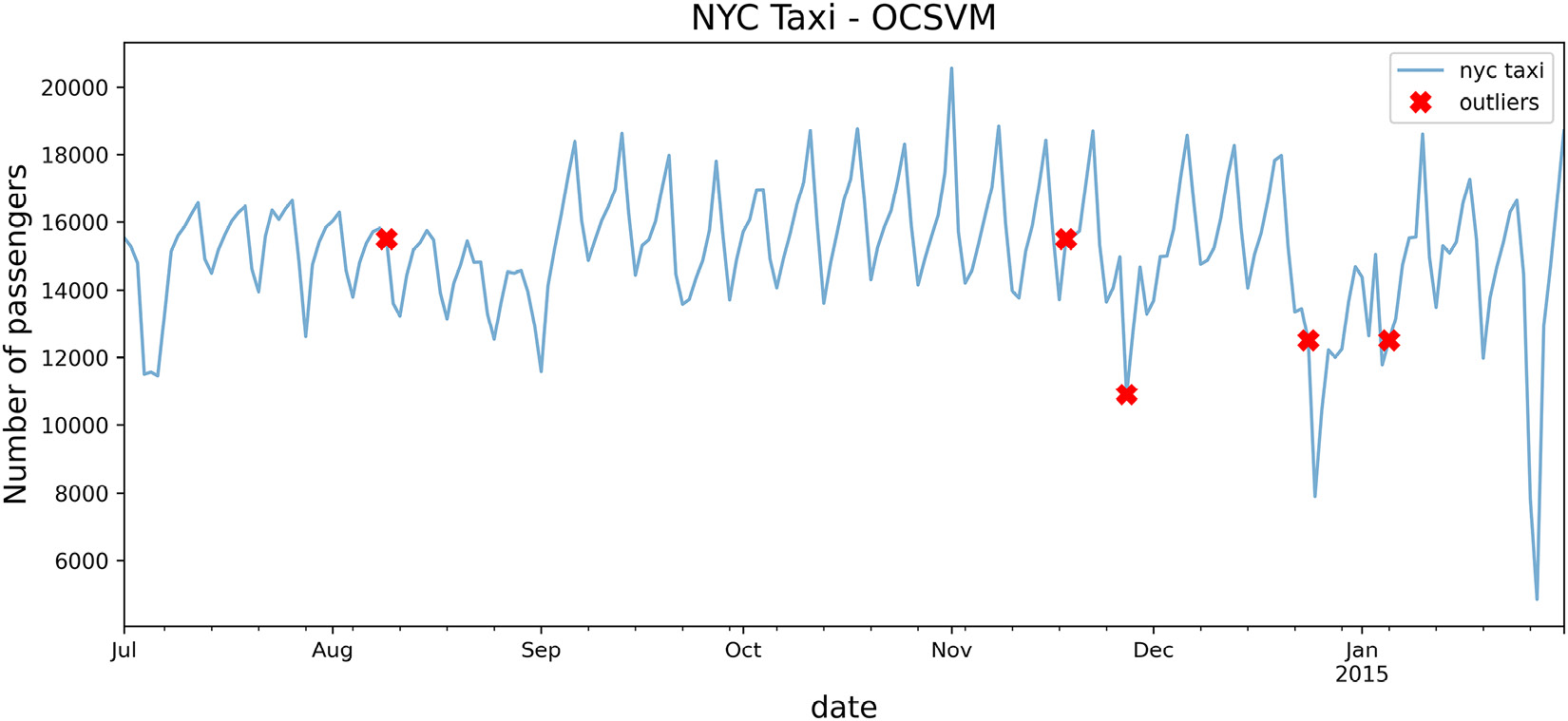
Figure 14.8 – Line plot with markers for each outlying point using OCSVM
When examining the plot in Figure 14.8, it is not clear why OCSVM picked up on those dates as being outliers. The RBF kernel can capture non-linear relationships, so you would expect it to be a robust kernel.
The reason for this inaccuracy is that SVM is sensitive to data scaling. To get better results, you will need to standardize (scale) your data first.
- Let's fix this issue and standardize the data and then rerun the algorithm again:
from pyod.utils.utility import standardizer
scaled = standardizer(tx)
predicted = pd.Series(ocsvm.fit_predict(scaled),
index=tx.index)
outliers = predicted[predicted == 1]
outliers = tx.loc[outliers.index]
outliers
>>
timestamp value
2014-07-06 11464.270833
2014-11-01 20553.500000
2014-11-27 10899.666667
2014-12-25 7902.125000
2014-12-26 10397.958333
2015-01-26 7818.979167
2015-01-27 4834.541667
Interestingly, now the model identified four out of the five known outlier dates.
The preceding code should produce a more reasonable plot, as shown in the following figure:
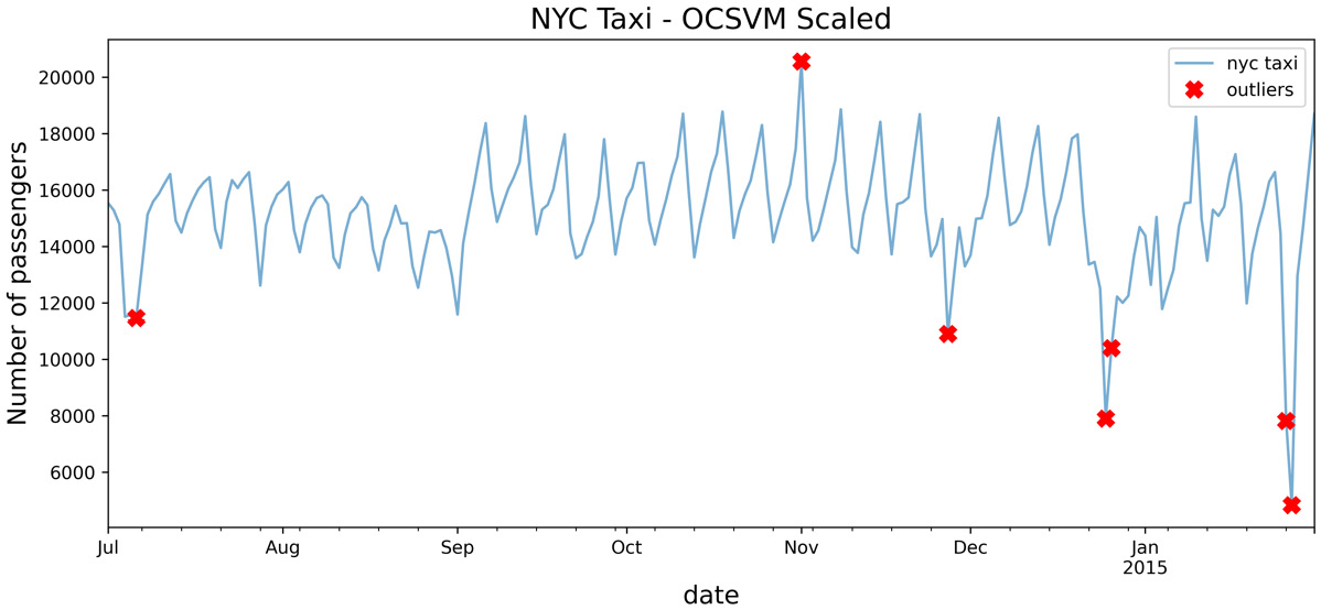
Figure 14.9 – OCSVM after scaling the data using the standardizer function
Compare the results from Figure 14.9 and Figure 14.8 to see how scaling made a big difference in how the OCSVM algorithm identified outliers.
How it works...
The PyOD implementation for OCSVM is a wrapper to scikit-learn's OneClassSVM implementation.
Similar to SVM, OneClassSVM is sensitive to outliers and also the scaling of the data. In order to get reasonable results, it is important to standardize (scale) your data before training your model.
There's more...
Let's explore how the different kernels perform on the same dataset. In the following code, you test four kernels: 'linear', 'poly', 'rbf', and 'sigmoid'.
Recall that when working with SVM, you will need to scale your data. You will use the scaled dataset created earlier:
for kernel in ['linear', 'poly', 'rbf', 'sigmoid']:
    ocsvm = OCSVM(contamination=0.03, kernel=kernel)
    predict = pd.Series(ocsvm.fit_predict(scaled),
                      index=tx.index, name=kernel)
    outliers = predict[predict == 1]
    outliers = tx.loc[outliers.index]
    plot_outliers(outliers, tx, kernel, labels=True)
The preceding code should produce a plot for each kernel so you can visually inspect and compare the difference between them:
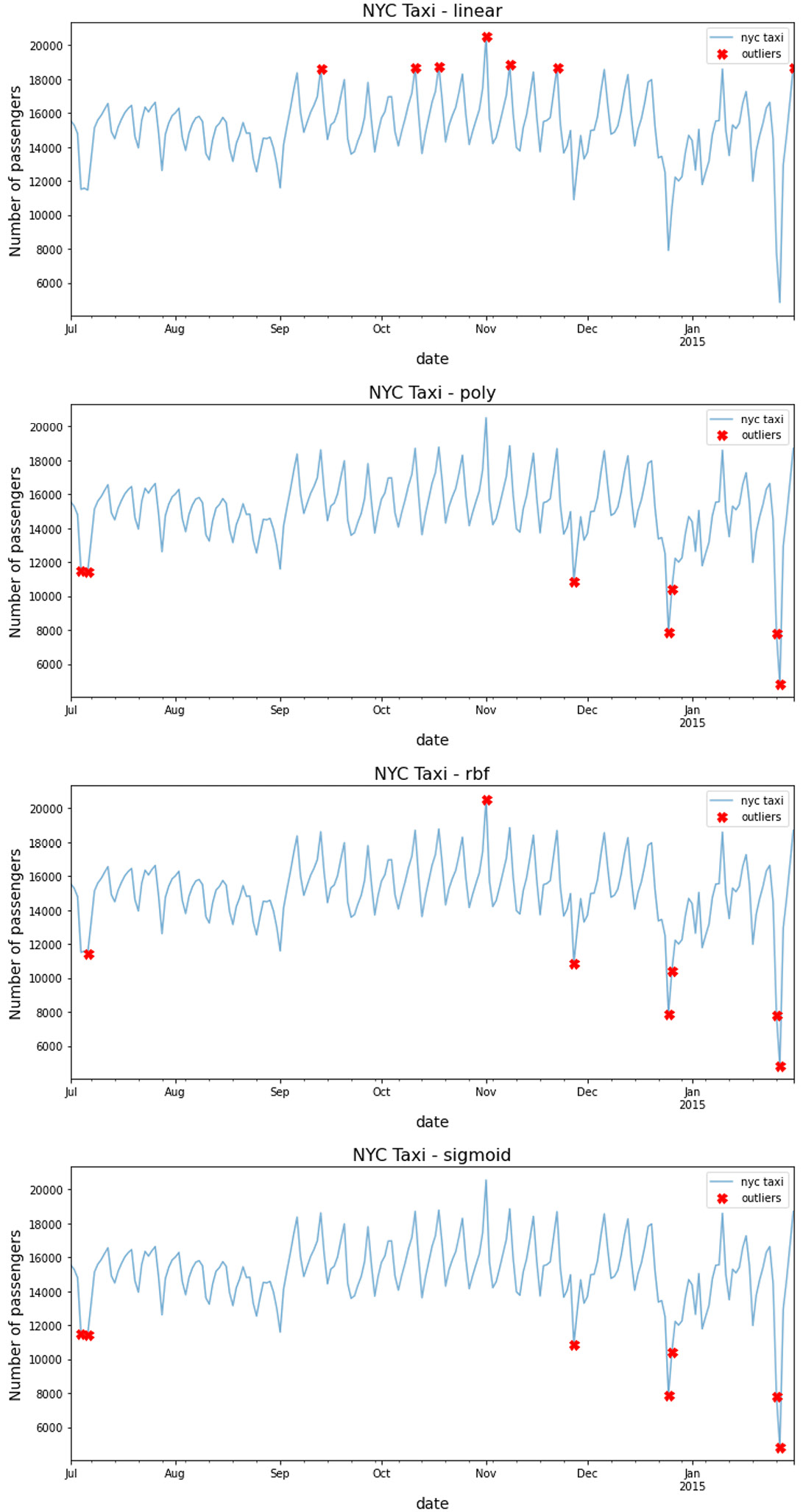
Figure 14.10 – Comparing the different kernels with OCSVM
Interestingly, each kernel method captured slightly different outliers. You can rerun the previous code to print out the labels (dates) for each marker by passing the labels=True parameter.
See also
To learn more about the OCSVM implementation, visit the official documentation here: https://pyod.readthedocs.io/en/latest/pyod.models.html#module-pyod.models.ocsvm.
Detecting outliers using COPOD
COPOD is an exciting algorithm based on a paper published in September 2020, which you can read here: https://arxiv.org/abs/2009.09463.
The PyOD library offers many algorithms based on the latest research papers, which can be broken down into linear models, proximity-based models, probabilistic models, ensembles, and neural networks.
COPOD falls under probabilistic models and is labeled as a parameter-free algorithm. The only parameter it takes is the contamination factor, which defaults to 0.1. The COPOD algorithm is inspired by statistical methods, making it a fast and highly interpretable model. The algorithm is based on copula, a function generally used to model dependence between independent random variables that are not necessarily normally distributed. In time series forecasting, copulas have been used in univariate and multivariate forecasting, which is popular in financial risk modeling. The term copula stems from the copula function joining (coupling) univariate marginal distributions to form a uniform multivariate distribution function.
How to do it...
In this recipe, you will continue to work with the tx DataFrame to detect outliers using the COPOD class from the PyOD library:
- Start by loading the COPOD class:
from pyod.models.copod import COPOD
- The only parameter you need to consider is contamination. Generally, think of this parameter (used in all the outlier detection implementations) as a threshold to control the model's sensitivity and minimize the false positives. Since it is a parameter you control, ideally, you want to run several models to experiment with the ideal threshold rate that works for your use cases.
For more insight into decision_scores_, threshold_, or predict_proba, please review the first recipe, Detecting outliers using KNN, of this chapter.
- Instantiate COPOD and update contamination to 0.03. Then, fit on the resampled data to train the model:
copod = COPOD(contamination=0.03)
copod.fit(tx)
>>
COPOD(contamination=0.03, n_jobs=1)
- Use the predict method to identify outliers. The method will output either 1 or 0 for each data point. For example, a value of 1 indicates an outlier.
Store the results in a pandas Series:
predicted = pd.Series(copod.predict(tx),
                      index=tx.index)
print('Number of outliers = ', predicted.sum())
>>
Number of outliers =  7
The number of outliers matches the number you got using iForest.
- Filter the predicted Series only to show the outlier values:
outliers = predicted[predicted == 1]
outliers = tx.loc[outliers.index]
outliers
>>
timestamp value
2014-07-04 11511.770833
2014-07-06 11464.270833
2014-11-27 10899.666667
2014-12-25 7902.125000
2014-12-26 10397.958333
2015-01-26 7818.979167
2015-01-27 4834.541667
Compared with other algorithms you have explored so far, you will notice some interesting outliers captured with COPOD that were not identified before. For example, COPOD identified July 4, a national holiday in the US (Independence Day). It happens to fall on a weekend (Friday being off). The COPOD model captured anomalies throughout the weekend for July 4 and July 6. It happens that July 6 was an interesting day due to a baseball game in New York.
- Use the plot_outliers function created in the Technical requirements section to visualize the output to gain better insights:
plot_outliers(outliers, tx, 'COPOD')
The preceding code should produce a plot similar to that in Figure 14.1, except the x markers are based on the outliers identified using the COPOD algorithm:
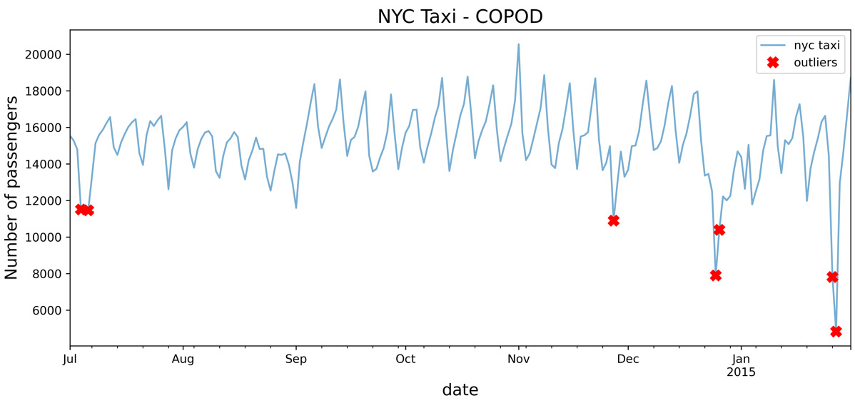
Figure 14.11 – Markers showing the identified potential outliers using the COPOD algorithm
To print the labels (dates) with the markers, just call the plot_outliers function again, but this time with labels=True:
plot_outliers(outliers, tx, 'COPOD', labels=True)
The preceding code should produce a similar plot to the one in Figure 14.11 with the addition of text labels.
How it works...
COPOD is an advanced algorithm, but it is still based on probabilistic modeling and finding statistically significant extremes within the data. Several tests using COPOD have demonstrated its superb performance against benchmark datasets. The appeal of using COPOD is that it is parameter-free (aside from the contamination factor). So, as a user, you do not have to worry about hyperparameter tuning.
There's more...
Another simple and popular probabilistic algorithm is the Median Absolute Deviation (MAD). We explored MAD in Chapter 8, Outlier Detection Using Statistical Methods, in the Outlier detection using modified z-score recipe, in which you built the algorithm from scratch.
This is a similar implementation provided by PyOD and takes one parameter, the threshold. If you recall from Chapter 8, Outlier Detection Using Statistical Methods, the threshold is based on the standard deviation.
The following code shows how we can implement MAD with PyOD. You will use threshold=3 to replicate what you did in Chapter 8, Outlier Detection Using Statistical Methods:
from pyod.models.mad import MAD
mad = MAD(threshold=3)
predicted = pd.Series(mad.fit_predict(tx),
                      index=tx.index)
outliers = predicted[predicted == 1]
outliers = tx.loc[outliers.index]
outliers
>>
timestamp  value
2014-11-01  20553.500000
2014-11-27  10899.666667
2014-12-25  7902.125000
2014-12-26  10397.958333
2015-01-26  7818.979167
2015-01-27  4834.541667
This should match the results you obtained in Chapter 8, Outlier Detection Using Statistical Methods, with the modified z-score implementation.
See also
To learn more about COPOD and its implementation in PyOD, visit the official documentation here: https://pyod.readthedocs.io/en/latest/pyod.models.html?highlight=copod#pyod.models.copod.COPOD.
If you are interested in reading the research paper for COPOD: Copula-Based Outlier Detection (published in September 2020), visit the arXiv.org page here: https://arxiv.org/abs/2009.09463.
Detecting outliers with PyCaret
In this recipe, you will explore PyCaret for outlier detection. PyCaret (https://pycaret.org) is positioned as "an open-source, low-code machine learning library in Python that automates machine learning workflows". PyCaret acts as a wrapper for PyOD, which you used earlier in the previous recipes for outlier detection. What PyCaret does is simplify the entire process for rapid prototyping and testing with a minimal amount of code.
You will use PyCaret to examine multiple outlier detection algorithms, similar to the ones you used in earlier recipes, and see how PyCaret simplifies the process for you.
Getting ready
The recommended way to explore PyCaret is to create a new virtual Python environment just for PyCaret so it can install all the required dependencies without any conflicts or issues with your current environment. If you need a quick refresher on how to create a virtual Python environment, check out the Development environment setup recipe, from Chapter 1, Getting Started with Time Series Analysis. The chapter covers two methods: using conda and venv.
The following instructions will show the process using conda. You can call the environment any name you like; for the following example, we will name our environment pycaret:
>> conda create -n pycaret python=3.8 -y
>> conda activate pycaret
>> pip install "pycaret[full]"
In order to make the new pycaret environment visible within Jupyter, you can run the following code:
python -m ipykernel install --user --name pycaret --display-name "PyCaret"
There is a separate Jupyter notebook for this recipe, which you can download from the GitHub repository:
How to do it...
In this recipe, you will not be introduced to any new concepts. The focus is to demonstrate how PyCaret can be a great starting point when you are experimenting and want to quickly evaluate different models. You will load PyCaret and run it for different outlier detection algorithms:
- Start by loading all the available functions from the pycaret.anomaly module:
from pycaret.anomaly import *
setup = setup(tx, session_id = 1, normalize=True)
This should display the following:
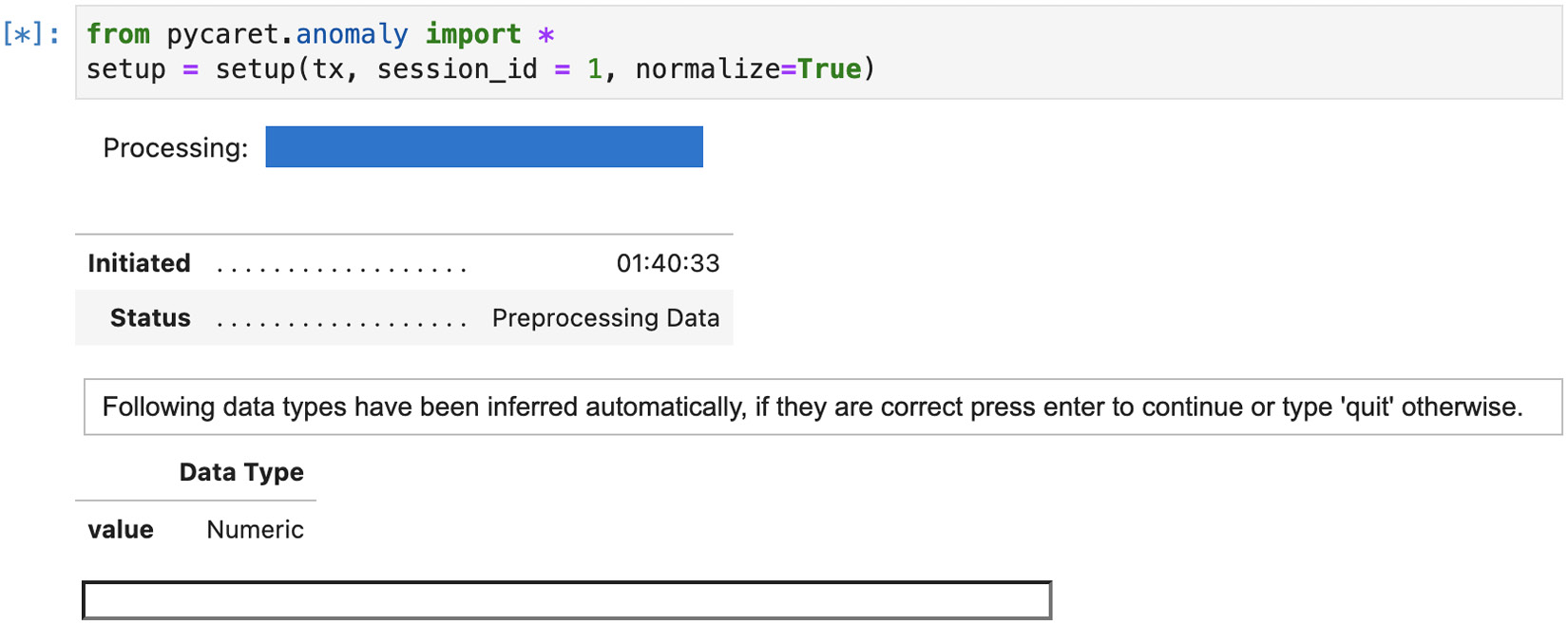
Figure 14.12 – Showing the initial screen in Jupyter Notebook/Lab pending user response
You will need to hit the Enter key to confirm and it will continue with the process. In the end, you see a long list of parameters (49 in total) and their default values. These parameters represent some of the preprocessing tasks that are automatically performed for you:
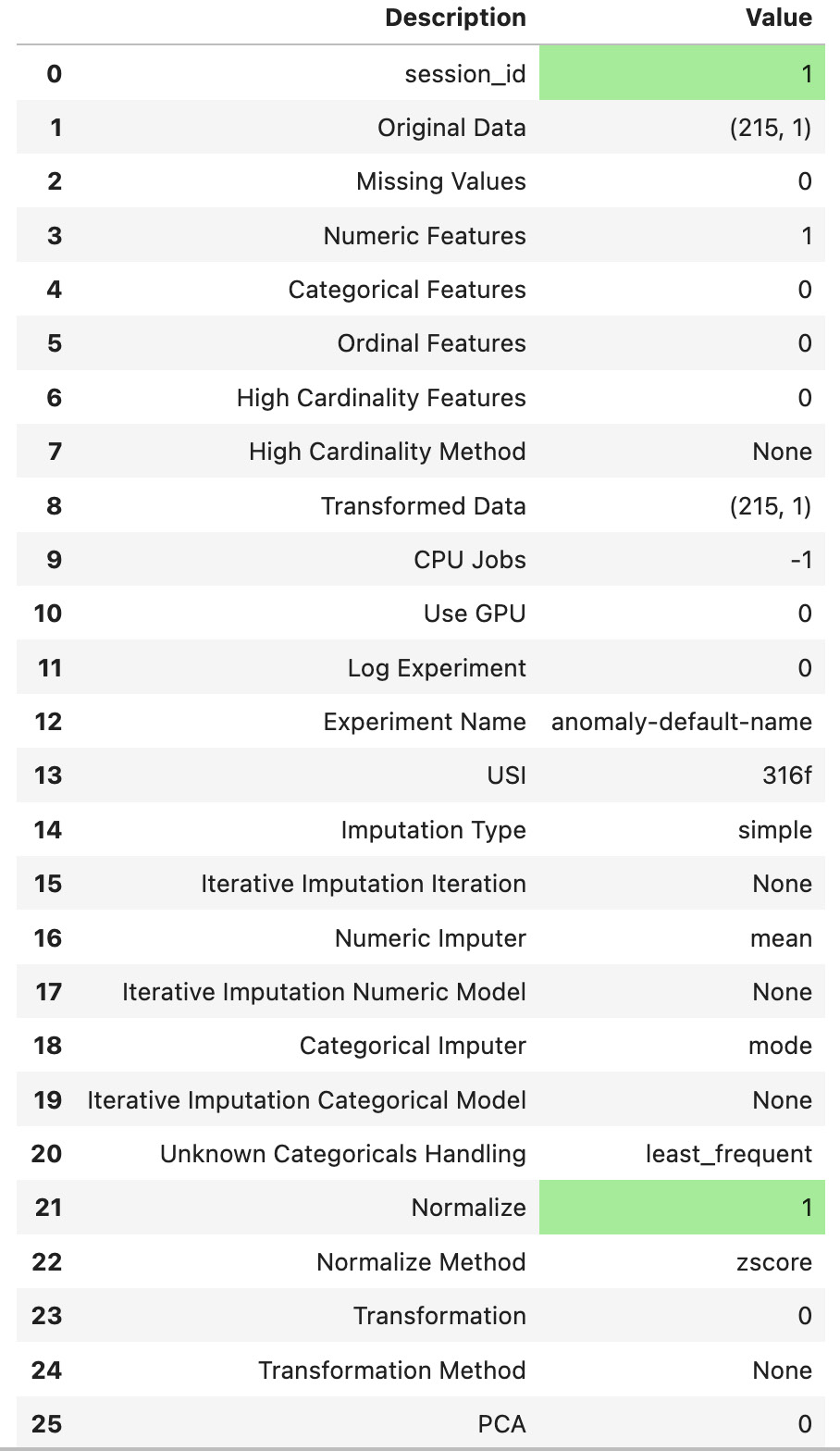
Figure 14.13 – The first 25 parameters and their values
This should display a pandas DataFrame, as follows:
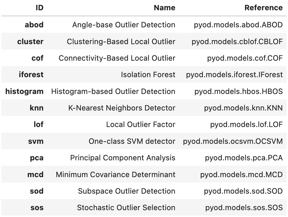
Figure 14.14 – Available outlier detection algorithms from PyCaret
Notice these are all sourced from the PyOD library. As stated earlier, PyCaret is a wrapper on top of PyOD and other libraries, such as scikit-learn.
- Let's store the names of the first eight algorithms in a list to use later:
list_of_models = models().index.tolist()[0:8]
list_of_models
>>
['abod', 'cluster', 'cof', 'iforest', 'histogram', 'knn', 'lof', 'svm']
- Loop through the list of algorithms and store the output in a dictionary so you can reference it later for your analysis. To create a model in PyCaret, you simply use the create_model() function. This is similar to the fit() function in scikit-learn and PyOD for training the model. Once the model is created, you can use the model to predict (identify) the outliers using the predict_model() function. PyCaret will produce a DataFrame with three columns: the original value column, a new column, Anomaly, which stores the outcome as either 0 or 1, where 1 indicates an outlier, and another new column, Anomaly_Score, which stores the score used (the higher the score, the higher the chance it is an anomaly).
You will only change the contamination parameter to match earlier recipes using PyOD. In PyCaret, the contamination parameter is called fraction and to be consistent, you will set that to 0.03 or 3% with fraction=0.03:
results = {}
for model in list_of_models:
    cols = ['value', 'Anomaly_Score']
    outlier_model = create_model(model, fraction=0.03)
    print(outlier_model)
    outliers = predict_model(outlier_model, data=tx)
    outliers = outliers[outliers['Anomaly'] == 1][cols]
    outliers.sort_values('Anomaly_Score', ascending=False, inplace=True)
    results[model] = {'data': outliers, 'model': outlier_model}
The results dictionary contains the output (a DataFrame) from each model.
- To print out the outliers from each model, you can simply loop through the dictionary:
for model in results:
print(f'Model: {model}')print(results[model]['data'], ' ')
This should print the results for each of the eight models. The following are the first two models from the list as an example:
Model: abod
                   value  Anomaly_Score
timestamp
2014-11-01  20553.500000      -0.002301
2015-01-27   4834.541667      -0.007914
2014-12-26  10397.958333      -3.417724
2015-01-26   7818.979167    -116.341395
2014-12-25   7902.125000    -117.582752
2014-11-27  10899.666667    -122.169590
2014-10-31  17473.354167   -2239.318906
Model: cluster
                   value  Anomaly_Score
timestamp
2015-01-27   4834.541667       3.657992
2015-01-26   7818.979167       2.113955
2014-12-25   7902.125000       2.070939
2014-11-01  20553.500000       0.998279
2014-12-26  10397.958333       0.779688
2014-11-27  10899.666667       0.520122
2014-11-28  12850.854167       0.382981
How it works...
PyCaret is a great library for automated machine learning, and recently they have been expanding their capabilities around time series analysis and forecasting and anomaly (outlier) detection. PyCaret is a wrapper over PyOD, the same library you used in earlier recipes of this chapter. Figure 14.14 shows the number of PyOD algorithms supported by PyCaret, which is a subset of the more extensive list from PyOD: https://pyod.readthedocs.io/en/latest/index.html#implemented-algorithms.
See also
To learn more about PyCaret's outlier detection, please visit the official documentation here: https://pycaret.gitbook.io/docs/get-started/quickstart#anomaly-detection.