Chapter 3: Data-Centric Approaches

In the Defining explanation methods and approaches section of Chapter 1, Foundational Concepts of Explainability Techniques, when we looked at the various dimensions of explainability, we discussed how data is one of the important dimensions. In fact, all machine learning (ML) algorithms depend on the underlying data being used.

In the previous chapter, we discussed various model explainability methods. Most of the methods discussed in Chapter 2, Model Explainability Methods, are model-centric. The concepts and ideas discussed were focused on making black-box models interpretable. But recently, the ML and AI communities have realized the core importance of data for any analysis or modeling purposes. So, more and more AI researchers are exploring new ideas and concepts around data-centric AI.

Since data plays a vital role in the model-building and prediction process, it is even more important for us to explain the functioning of any ML and AI algorithm with respect to the underlying data. From what I have observed from my experience in this field, the failure of any ML systems in production happens neither due to the poor choice of ML algorithm nor due to an inefficient model training or tuning process, but rather it occurs mostly due to inconsistencies in the underlying dataset. So, this chapter focuses on the concepts of data-centric explainable AI (XAI).

The goal of this chapter is to introduce you to the concepts of data-centric XAI. After reading this chapter, you will get to know about the various methods that can be performed to check the quality of the data, which might influence the model outcome. For production-level ML systems, the inference data can have issues related to its consistency and quality. So, monitoring these drifts is extremely important. Additionally, there can be external noise or perturbations affecting the data that can impact the model. So, these are some data-centric approaches that we will be discussing that are used for explaining ML models. In this chapter, the following main topics will be covered:

• Introduction to data-centric XAI
• Thorough data analysis and profiling processes
• Monitoring and anticipating drifts
• Checking adversarial robustness
• Measuring data forecastability

Now, let's dive in!

Technical requirements

Similar to Chapter 2, Model Explainability Methods, for this chapter, certain tutorial examples to implement some of the techniques to perform data-centric XAI in Python on certain interesting datasets have been provided. We will be using Python Jupyter notebooks to run the code and visualize the output throughout this book. The code and dataset resources for this chapter can be downloaded or cloned from the following GitHub repository: https://github.com/PacktPublishing/Applied-Machine-Learning-Explainability-Techniques/tree/main/Chapter03. Other important Python frameworks required to run the code will be mentioned in the notebooks with other relevant details to understand the code implementation of these concepts. Other important Python frameworks required to run the code will be mentioned in the notebooks along with other relevant details to understand the code implementation of these concepts. Please note that this chapter mainly focuses on providing a conceptual understanding of the topics covered. The Jupyter notebooks will help you gain the supplementary knowledge that is required to implement these concepts in practice. I recommend that you first read this chapter and then work on executing the Jupyter notebooks.

Introduction to data-centric XAI

Andrew Ng, one of the influential thought leaders in the field of AI and ML, has often highlighted the importance of using a systematic approach to build AI systems with high-quality data. He is one of the pioneers of the idea of data-centric AI, which focuses on developing systematic processes to develop models using clean, consistent, and reliable data, instead of focusing on the code and the algorithm. If the data is consistent, unambiguous, balanced, and available in sufficient quantity, this leads to faster model building, improved accuracy, and faster deployment for any production-level system.

Unfortunately, all AI and ML systems that exist in production today are not in alignment with the principles of data-centric AI. Consequently, there can be severe issues with the underlying data that seldom get detected but eventually lead to the failure of ML systems. That is why data-centric XAI is important to inspect and evaluate the quality of the data being used.

When we talk about explaining the functioning of any black-box model with respect to the data, we should inspect the volume of the data, the consistency of the data (particularly for supervised ML problems), and the purity and integrity of the data. Now, let's discuss these important aspects of data-centric XAI and understand why they are important.

Analyzing data volume

One of the classical problems of ML algorithms is the lack of generalization due to overfitting. Overfitting can be reduced by adding more data or by getting datasets of the appropriate volume to solve the underlying problem. So, the very first question we should ask about the data to explain the black-box model is "Is the model trained on sufficient data?" But for any industrial application, since data is very expensive, adding more data is not always feasible. So, the question should be "How do we find out if the model was trained on sufficient data?"

One way to inspect whether the model was trained on sufficient data is by training models with 70%, 80%, and 90% of the training dataset. If the model accuracy shows an increasing trend, with an increase in the volume of the data, that means the volume of the data can influence the model's performance. If the accuracy of the trained model, which has been trained on the entire training dataset, is low, then an increasing trend of model accuracy with increasing data volume indicates that the model is not trained on sufficient data. Therefore, more data is needed to make the model more accurate and generalized.

For production systems, if data is continuously flowing and there is no constraint on the availability of data, continuous training and monitoring of the models should be done on changing volumes of the data to understand and analyze its impact on the overall model performance.

Analyzing data consistency

Data consistency is another important factor to inspect when explaining ML models with respect to the data. One of the fundamental steps of analyzing data consistency is by understanding the distribution of the data. If the data is not evenly distributed, if there is a class imbalance, or if the data is skewed toward a particular direction, it is very likely that the model will be biased or less efficient for a particular segment of the data.

For production systems, it has been often observed that the inference data used in the production application might have some variance with the data used during training and validation. This phenomenon is known as data drift, and it refers to an unexpected change in the data structure or the statistical properties of the dataset, thus making the data corrupt and hampering the functioning of the ML system.

Data drift is very common for most real-time predictive models. This is simply because, in most situations, the data distribution changes over a period of time. This can happen due to a variety of reasons, for instance, if the system through which the data is being collected (for example, sensors) starts malfunctioning or needs to be recalibrated, then data drift can occur. Other external factors such as the surrounding temperature and surrounding noise can also introduce data drift. There can be a natural change in the relationship between the features that might cause data to drift. Consequently, if the training data is significantly different from the inference data, the model will make an error when predicting the outcome.

Now, sometimes, there can be a drift in the whole dataset or there can be a drift in one or more features. If there is a drift in a single feature, this is referred to as feature drift. There are multiple ways to detect feature drift such as the Population Stability Index (PSI) (https://www.lexjansen.com/wuss/2017/47_Final_Paper_PDF.pdf), Kullback–Leibler Divergence (KL Divergence) (https://www.countbayesie.com/blog/2017/5/9/kullback-leibler-divergence-explained), and Wasserstein metric (Earth Movers Distance) (http://infolab.stanford.edu/pub/cstr/reports/cs/tr/99/1620/CS-TR-99-1620.ch4.pdf). The application of some of these techniques has been demonstrated at https://github.com/PacktPublishing/Applied-Machine-Learning-Explainability-Techniques/tree/main/Chapter03. These statistical methods are popular ways to measure the distance between two data distributions. So, if the distance is significantly large, this is an indication of the presence of drift.

Apart from feature drift, Label Drift or Concept Drift can occur if the statistical properties of the target variable change over a period of time due to unknown reasons. However, overall data consistency is an important parameter for root cause analysis inspection when interpreting black-box models.

Analyzing data purity

The datasets used for practical industrial problems are never clean, even though most organizations spend a significant amount of time and investment on data engineering and data curation to drive a culture of data-driven decision-making. Yet, almost all practical datasets are messy and require a systematic approach to curation and preparation.

When we train a model, usually, we put our efforts into data preprocessing and preparation steps such as finding duplicates or unique values, removing noise or unwanted values from the data, detecting outliers, handling missing values, handling features with mixed data types, and even transforming raw features or feature engineering to get better ML models. On a high level, these methods are meant for removing impurities from the training data. But what if a black-box ML model is trained on a dataset with less purity and, hence, performs poorly?

That is why analyzing data purity is an important step in data-centric XAI. Aside from the data preprocessing and preparation methods mentioned earlier, there are other data integrity issues that exist as follows:

• Label ambiguity: For supervised ML problems, label ambiguity can be a very critical problem. If two or more instances of a dataset, which are very similar, have multiple labels, then this can lead to label ambiguity. Ambiguous labeling of the target variable can increase the difficulty of even domain experts classifying the samples correctly. Label ambiguity can be a very common problem, as, usually, labeled datasets are prepared by human subject-matter experts who are prone to human error.
• Dominating features frequency change (DFCC): Inspecting DFFC in the training and inference dataset is another parameter that can cause data integrity issues. In Chapter 2, Model Explainability Methods, when we discussed feature importance, we understood that not all features within the dataset are equally important, and some of the features have more influential power on the model's decision-making process. These are the dominating features in the dataset, and if the variance in the values of the dominating features in the training and the inference dataset is high, it is very likely that the model will make errors when predicting the outcome.

Other data purity issues, such as the introduction of a new label or new feature category, or out of bound values (or anomalies) for a particular feature in the inference set, can cause the failure of ML systems in production.

The following table shows certain important data purity checks that can be performed using the Deepchecks Python framework:

Figure 3.1 – Data purity checks using the Deepchecks framework

Data-centric XAI also includes other parameters that can be analyzed such as adversarial robustness (https://adversarial-ml-tutorial.org/introduction/), the trust score comparison (https://arxiv.org/abs/1805.11783), covariate shift (https://arxiv.org/abs/2111.08234), data leakage between the training and validation datasets (https://machinelearningmastery.com/data-leakage-machine-learning/), and model performance sensitivity analysis based on data alterations. All of these concepts apply to both tabular data and unstructured data such as images and text.

To explore practical ways of data purity analysis, you can refer to the Jupyter notebook at https://github.com/PacktPublishing/Applied-Machine-Learning-Explainability-Techniques/blob/main/Chapter03/Data_Centric_XAI_part_1.ipynb. We will discuss these topics later in the chapter.

Thorough data analysis and profiling process

In the previous section, you were introduced to the concept of data-centric XAI in which we discussed three important aspects of data-centric XAI: analyzing data volume, data consistency, and data purity. You might already be aware of some of the methods of data analysis and data profiling that we are going to learn in this section. But we are going to assume that we already have a trained ML model and, now, we are working toward explaining the model's decision-making process by adopting data-centric approaches.

The need for data analysis and profiling processes

In Chapter 2, Model Explainability Methods, when we discussed knowledge extraction using exploratory data analysis (EDA), we discovered that this was a pre-hoc analysis process, in which we try to understand the data to form relevant hypotheses. As data scientists, these initial hypotheses are important as they allow us to take the necessary steps to build a better model. But let's suppose that we have a baseline trained ML model and the model is not performing as expected because it is not meeting the benchmark accuracy scores that were set.

Following the principles of model-centric approaches, most data scientists might want to spend more time in hyperparameter tuning, training for a greater number of epochs, feature engineering, or choosing a more complex algorithm. After a certain point, these methods will become limited and provide a very small boost to the model's accuracy. That is when data-centric approaches prove to be very efficient.

Data analysis as a precautionary step

By the principles of data-centric explainability approaches, at first, we try to perform a thorough analysis of the underlying dataset. We try to randomly reshuffle the data to create different training and validation sets and observe any overfitting or underfitting effects. If the model is overfitting or underfitting, clearly more data is required to generalize the model. If the available data is not sufficient in volume, there are ways to generate synthetic or artificial data. One such popular technique used for image classification is data augmentation (https://research.aimultiple.com/data-augmentation/). The synthetic minority oversampling technique (SMOTE) (https://machinelearningmastery.com/smote-oversampling-for-imbalanced-classification/) is also a powerful method that you can use to increase the size of the dataset. Some of these data-centric approaches are usually practiced during conventional ML workflows. However, we need to realize the importance of these steps for the explainability of black-box models.

Once we have done enough tests to understand whether the volume of the data is sufficient, we can try to inspect the consistency and purity of the data at a segmented level. If we are working on a classification problem, we can try to understand whether the model performance is consistent for all the classes. If not, we can isolate the particular class or classes for which the model performance is poor. Then, we check for data drifts, feature drifts, concept drifts, label ambiguity, data leakage (for example, when unseen test data trickles into the training data), and other data integrity checks for that particular class (or classes). Usually, if there is any abnormality with the data for a particular class (or classes), these checks are sufficient to isolate the problem. A thorough data analysis acts as a precautionary step to detect any loopholes in the modeling process.

Building robust data profiles

Another approach is to build statistical profiles of the data and then compare the profiles between the training data and the inference data. A statistical profile of a dataset is a collection of certain statistical measures of its feature values segmented by the target variable class (or, in the case of a regression problem, the bin of values). The selection of the statistical measures might change from use case to use case, but usually, I select statistical measures such as the mean, median, average variance, average standard deviation, coefficient of variation (standard deviation/mean), and z-scores ((value – mean)/standard deviation) for creating data profiles. In the case of time series data, measures such as the moving average and the moving median can also be very important.

Next, let's try to understand how this approach is useful. Suppose there is an arbitrary dataset that has three classes (namely class 0, 1, and 2) and only two features: feature 1 and feature 2. When we try to prepare the statistical profile, we would try to calculate certain statistical measures (such as the mean, median, and average variance in this example) for each feature and each class.

So, for class 0, a set of profile values consisting of the mean of feature 1, the median of feature 1, the average variance of feature 1, the mean of feature 2, the median of feature 2, and the average variance of feature 2 will be generated. Similarly, for class 1 and class 2, a set of profile values will be created for each class. The following table represents the statistical profile of the arbitrary dataset that we have considered for this example:

Figure 3.2 – A table showing a statistical profile segmented by each class for an arbitrary dataset

These statistical measures of the feature values can be used to compare the different classes. If a trained model predicts a particular class, we can compare the feature values with the statistical profile values for that particular class to get a fair idea about the influential features contributing to the decision-making process of the model. But more importantly, we can create separate statistical profiles for the validation set, test set, and inference data used in the production systems and compare them with the statistical profile of the training set. If the absolute percentage change between the values is significantly higher (say, > 20%), then this indicates the presence of data drift.

In our example, let's suppose that if the absolute percentage change in the average variance score for feature 1 for class 1 is about 25% between the training data and the inference data, then we have a feature drift for feature 1, and this might lead to poor model performance with the inference data for the production systems. Statistical profiles can also be created for unstructured data such as images and text, although the choice of statistical measures might be slightly complicated.

In general, this approach is very easy to implement and it helps us to validate whether the data used for training a model and the data used during testing or inference are consistent or not, which is an important step for data-centric model explainability. In the next section, we will discuss about the importance of monitoring and anticipating drifts for explaining ML systems.

Monitoring and anticipating drifts

In the previous section, we understood how a thorough data analysis and data profiling approach can help us to identify data issues related to volume, consistency, and purity. Usually, during the initial data exploration process, most data scientists try to inspect issues in the dataset in terms of volume and purity and perform necessary preprocessing and feature engineering steps to handle these issues.

But the detection of data consistency for real-time systems and production systems is a challenging problem for almost all ML systems. Additionally, issues relating to data consistency are often overlooked and are quite unpredictable as they can happen at any point in time in production systems. Some of the cases where data consistency issues can occur are listed as follows:

• They can occur due to natural reasons such as changes in external environmental conditions or due to the natural wear and tear of sensors or systems capturing the inference data.
• They can happen due to human-induced reasons such as any physical damage caused to the system collecting the data, any bug in the software program running the algorithm due to which the input data is being transformed incorrectly, or any noise introduced to the system while upgrading an older version of the system.

So, all of these situations can introduce data drifts and concept drifts, which eventually lead to the poor performance of ML models. And since drifts are very common in reality, issues related to drifts should be pre-anticipated and should be considered during the design process of any ML system.

Detecting drifts

After trained models are deployed for any production ML system, performance monitoring and feedback based on model performance is a necessary process. As we monitor the model performance, checking for any data or concept drifts is also critical in this step. At this point, you might be wondering two things:

• What is the best way to identify the presence of a drift?
• What happens when we detect the presence of a drift?

As discussed in the Analyzing data consistency section, there are two types of data drifts – feature drifts and concept drifts. Feature drifts happen when the statistical properties of the features or the independent variables change due to an unforeseen reason. In comparison, concept drift occurs when the target class variable, which the model is trying to predict, changes its initial relationship with the input features in a dynamic setting. In both cases, there is a statistical change in the underlying data. So, my recommendation for detecting drifts is to use the data profiling method discussed in the previous section.

A real-time monitoring dashboard is always helpful for any real-time application to monitor any drift. In the dashboard, try to have necessary visualizations for each class and each feature, comparing the statistical profile values with the actual live values flowing into the trained model.

Particularly for concept drifts, comparing the correlations of the features with the target outcome is extremely helpful. Since drifts can arise after a certain period of time or even during a specific point in time due to external reasons, it is always advisable to monitor the statistical properties of the inference data in a time window period (for instance, for 50 consecutive data points or 100 consecutive data points) rather than a continuous cumulative basis. For the purposes of feedback, necessary alerts and triggers can be set when abnormal data points are detected in the inference data, which might indicate the presence of data drift.

Selection of statistical measures

Sometimes, the selection of statistical measures can be difficult. So, we usually go for some popular distribution metrics to detect the presence of data drift using a quantitative approach. One such metric is called trust score distribution (https://arxiv.org/abs/1805.11783).

The following diagram shows the trust score distribution plot obtained using the Deepchecks Python framework:

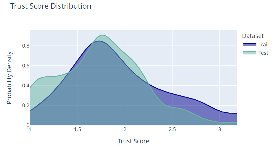
Figure 3.3 – An example of the trust score distribution between the training dataset and the inference dataset

Trust score is a distribution metric used to measure the agreement between the ML classifier on the training set and an updated k-Nearest Neighbor (kNN) classifier on the inference dataset. The preceding diagram shows a trust score distribution plot between the training dataset and the inference dataset.

Ideally, the distributions should be almost the same for both the train and test datasets. However, if the trust score distribution for the inference set is skewed toward the extreme left, this indicates that the trained model has less confidence in the inference data, thereby alluding to the presence of drift. If the distribution of the trust score on the inference data is skewed toward the extreme right, there might be some problem with the model and there is a high probability of data leakage, as ideally, the trained model cannot be more confident in the test data in comparison to the training data.

To detect feature drifts on categorical features, the popular choice of metric is the population stability index (PSI) (https://www.lexjansen.com/wuss/2017/47_Final_Paper_PDF.pdf). This is a statistical method used to measure the shift in a variable over a period of time. If the overall drift score is more than 0.2 or 20%, then the drift is considered to be significant, establishing the presence of feature drift.

To detect feature drifts in numeric features, the Wasserstein metric (https://kowshikchilamkurthy.medium.com/wasserstein-distance-contraction-mapping-and-modern-rl-theory-93ef740ae867) is the popular choice. This is a distance function for measuring the distance between two probability distributions. Similar to PSI, if the drift score using the Wasserstein metric is higher than 20%, this is considered to be significant and the numerical feature is considered to have feature drift.

The following diagram illustrates feature drift estimation using the Wasserstein (Earth Mover's) distance and Predictive Power Score (PPS) with the Deepchecks framework:

Figure 3.4 – Feature drift estimation using Wasserstein (Earth Mover's) distance and PPS of features

Similar concept drifts can also be detected using these metrics. For regression problems, the Wasserstein metric is effective, while for classification problems PSI is more effective. You can see the application of these methods on a practical dataset at https://github.com/PacktPublishing/Applied-Machine-Learning-Explainability-Techniques/tree/main/Chapter03. Additionally, there are other statistical methods that are extremely useful for detecting data drifts such as Kullback-Leibler Divergence (KL Divergence), the Bhattacharyya distance, Jensen-Shannon Divergence (JS Divergence), and more.

In this chapter, our focus is not on learning these metrics, but I strongly recommend you to take a look at the Reference section to find out more about these metrics and their application for finding data drifts. These methods are also applicable to images. Instead of structured feature values, the distributions of the pixel intensity value of the image datasets are used to detect drifts.

Now that we are aware of certain effective ways in which to detect drifts, what do we do when we have identified the presence of drifts? The first step is to alert our stakeholders if the ML system is already in production. Incorrect predictions due to data drift can impact many end users, which might, ultimately, lead to the loss of trust of the end users. The next step is to check whether the drift is temporary, seasonal, or permanent in nature. Analysis of the nature of the drift can be challenging, but if the changes that are causing the drift can be identified and reverted, then that is the best solution.

If the drift is temporary, the first step is to identify the temporary change that caused the drift and then revert the changes. For seasonal drifts, seasonal changes to the data should be accounted for during the training process or as an additional preprocessing step to normalize any seasonal effects on the data. This is so that the model is aware of the seasonal pattern in the data. However, if the drift is permanent, then the only option is to retrain the model on the new data and deploy the newly trained model for the production system.

In the context of XAI, the detection of drifts can justify the failure of any ML model or algorithm and helps to improve the model by identifying the root cause of the failure. In the next section, we will discuss another data-centric quality inspection step that can be performed to ensure the robustness of ML models.

Checking adversarial robustness

In the previous section, we discussed the importance of anticipating and monitoring drifts for any production-level ML system. Usually, this type of monitoring is done after the model has been deployed in production. But even before the model is deployed in production, it is extremely critical to check for the adversarial robustness of the model.

Most ML models are prone to adversarial attacks or an injection of noise to the input data, causing the model to fail by making incorrect predictions. The degree of adversarial attacks increases with the model's complexity, as complex models are very sensitive to noisy data samples. So, checking for adversarial robustness is about evaluating how sensitive the trained model is toward adversarial attacks.

In this section, first, we will try to understand the impact of adversarial attacks on the model and why this is important in the context of XAI. Then, we will discuss certain techniques that we can use to increase the adversarial robustness of ML models. Finally, we will discuss the methods that are used to evaluate the adversarial robustness of models, which can be performed as an exercise before deploying ML models into production, and how this forms a vital part of explainable ML systems.

Impact of adversarial attacks

Over the past few years, adversarial attacks have been a cause of great concern for the AI community. These attacks can inject noise to modify the input data in such a way that a human observer can easily identify the correct outcome but an ML model can be easily fooled and start predicting completely incorrect outcomes. The extent of the attack depends on the attacker's access to the model.

Usually, in production systems, the trained model (especially the model parameters) is fixed and cannot be modified. But the inference data flowing into the model can be polluted with abrupt noise signals, thus making the model misclassify. Human experts are extremely efficient in filtering out the injected noise, but ML models fail to isolate the noise from the actual data if the model has not been exposed to such noisy samples during the training phase. Sometimes, these attacks can be targeted attacks, too.

For example, if a face recognition system allows access to only a specific person, adversarial attacks can modify the image of any person to a specific person by introducing some noise. In this case, an adversarial algorithm would have to be trained using the target sample to construct the noise signal. There are other forms of adversarial attacks as well, which can modify the model during the training phase itself. However, since we are discussing this in the context of XAI, we will concentrate on the impact of adversarial effects on trained ML models.

There are different types of adversarial attacks that can impact trained ML models:

• Fast Gradient Sign Method (FGSM): FGSM is one such method that uses gradients of deep learning models to learn adversarial samples. For image classifiers, this can be a common problem, as FGSM creates perturbations on the pixel values of an image by adding or subtracting pixel intensity values depending on the direction of the gradient descent of the model. This can fool the model to misclassify and severely affect the performance of the model, but it does not create any problem for a human observer. Even if the modification appears to be negligible, the method adds an evenly distributed noise that is enough to cause the misclassifications.
• The Carlini & Wagner (C&W) attack: Another common adversarial attack is the C&W attack. This method uses the three norm-based distance metrics (, , and ) to find adversarial examples, such that the distance between the adversarial example and the original sample is minimal. Detecting C&W attacks is more difficult than FGSM attacks.
• Targeted adversarial patch attacks: Sometimes, injecting noise (that is, the addition of noisy random pixels) into the entire image is not necessary. The addition of a noisy image segment to only a small portion of the image can be equally harmful to the model. Targeted adversarial patch attacks can generate a small adversarial patch that is then superimposed with the original sample, thus occluding the key features of the data and making the model classify incorrectly. There are other forms of adversarial attacks too, and many more new methods can be discovered in the future. However, the impact will still be the same.

The following diagram shows how different adversarial attacks can introduce noise in an image, thereby making it difficult for the model to give correct predictions. Despite the addition of noise, we, as human beings, can still predict the correct outcome, but the trained model is completely fooled by adversarial attacks:

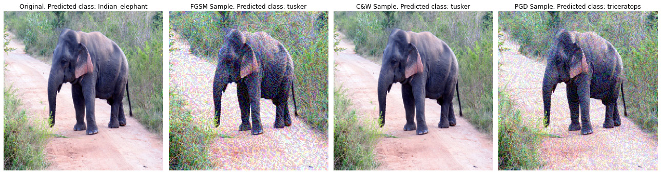
Figure 3.5 – Adversarial attacks on the inference data leading to incorrect model predictions

Adversarial attacks can force an ML model to produce incorrect outcomes that can severely affect end users. In the next section, let's try to explore ways to increase the adversarial robustness of models.

Methods to increase adversarial robustness

In production systems, adversarial attacks can mostly inject noise into the inference data. So, to reduce the impact of adversarial attacks, we would either need to teach the model to filter out the noise or expose the presence of noisy samples during the training process or train the models to detect adversarial samples:

• The easiest option is to filter out the noise as a defense mechanism to increase the adversarial robustness of ML models. Any adversarial noise results in an abrupt change in the input samples. In order to filter out any abrupt change from any signal, we usually try to apply a smoothing filter such as Spatial smoothing. Spatial smoothing is equivalent to the blurring operation in images and is used to reduce the impact of the adversarial attack. From experience, I have observed that an adaptive median spatial smoothing (https://homepages.inf.ed.ac.uk/rbf/HIPR2/median.htm), which works at a local level through a windowing approach is more effective than smoothing at a global level. The statistical measure of the median is always more effective in filtering out noise or outliers from the data.
• Another approach to increase adversarial robustness is by introducing adversarial examples during the training process. By using the technique of data augmentation, we can generate adversarial samples from the original data and include the augmented data during the training process. If training the model from scratch using augmented adversarial samples is not feasible, then the trained ML model can actually be fine-tuned on the adversarial samples using transfer learning. Here, the trained model weights can be taken to be fine-tuned on the newer samples.
• The process of training a model with adversarial samples is often referred to as adversarial training. We can even train a separate model using adversarial training, just to detect adversarial samples from original samples, and use it along with the main model to trigger alerts if adversarial samples are generated. The idea of exposing the model to possible adversarial samples is similar to the idea of stress testing in cyber security (https://ieeexplore.ieee.org/document/6459909).

Figure 3.6 illustrates how spatial smoothing can be used as a defense mechanism to minimize the impact of adversarial attacks:

Figure 3.6 – Using spatial smoothing as a defense mechanism to minimize the impact of adversarial attacks

Using the methods that we have discussed so far, we can increase the adversarial robustness of trained ML models to a great extent. In the next section, we will try to explore ways to evaluate the adversarial robustness of ML models.

Evaluating adversarial robustness

Now that we have learned certain approaches in which to defend against adversarial attacks, the immediate question that might come to mind is how can we measure the adversarial robustness of models?

Unfortunately, I have never come across any dedicated metric to quantitatively measure the adversarial robustness of ML models, but it is an important research topic for the AI community. The most common approaches by which data scientists evaluate the adversarial robustness of ML models are stress testing and segmented stress testing:

• In stress testing, adversarial examples are generated by FGSM or C&W methods. Following this, the model's accuracy is measured on the adversarial examples and compared to the model accuracy obtained with the original data. The strength of the adversarial attack can also be increased or decreased to observe the variation of the model performance with the attack strength. Sometimes, a particular class or feature can become more vulnerable to adversarial attacks than the entire dataset. In those scenarios, segmented stress testing is beneficial.
• In segmented stress testing, instead of measuring the adversarial robustness of the entire model on the entire dataset, segments of the dataset (either for specific classes or for specific features) are considered to compare the model robustness with the adversarial attack strengths. Adversarial examples can be generated with random noise or with Gaussian noise. For certain datasets, quantitative metrics such as the Peak Signal-to-Noise ratio (PSNR) (https://www.ni.com/nl-be/innovations/white-papers/11/peak-signal-to-noise-ratio-as-an-image-quality-metric.html) and Erreur Relative Globale Adimensionnelle de Synthese (ERGAS) (https://www.researchgate.net/figure/Erreur-Relative-Globale-Adimensionnelle-de-Synthese-ERGAS-values-of-fused-images_tbl1_248978216) are used to measure the data or signal quality. Otherwise, the adversarial robustness of ML models can be quantitatively inspected by the model's prediction of adversarial samples.

More than the method of evaluating adversarial robustness, inspecting adversarial robustness and monitoring the detection of adversarial attacks is an essential part of explainable ML systems. Next, let's discuss the importance of measuring data forecastability as a method to provide data-centric model explainability.

Measuring data forecastability

So far, we have learned about the importance of analyzing data by inspecting its consistency and purity, looking for monitoring drifts, and checking for any adversarial attacks to explain the working of ML models. But some datasets are extremely complex and, hence, training accurate models even with complex algorithms is not feasible. If the trained model is not accurate, it is prone to make incorrect predictions. Now the question is how do we gain the trust of our end users if we know that the trained model is not extremely accurate in making the correct predictions?

I would say that the best way to gain trust is by being transparent and clearly communicating what is feasible. So, measuring data forecastability and communicating the model's efficiency to end users helps to set the right expectation.

Data forecastability is an estimation of the model's performance using the underlying data. For example, let's suppose we have a model to predict the stock price of a particular company. The stock price data that is being modeled by the ML algorithm can predict the stock price with a maximum of 60% accuracy. Beyond that point, it is not practically possible to generate a more accurate outcome using the given dataset.

But let's say that if other external factors are considered to supplement the current data, the model's accuracy can be boosted. This proves that it is not the ML algorithm that is limiting the performance of the system, but rather the dataset that is used for modeling does not have sufficient information to get a better model performance. Hence, it is a limitation of the dataset that can be estimated by measure of data forecastability.

The following diagram shows a number of model evaluation visualizations that can be used to analyze data forecastability using the Deepchecks framework:

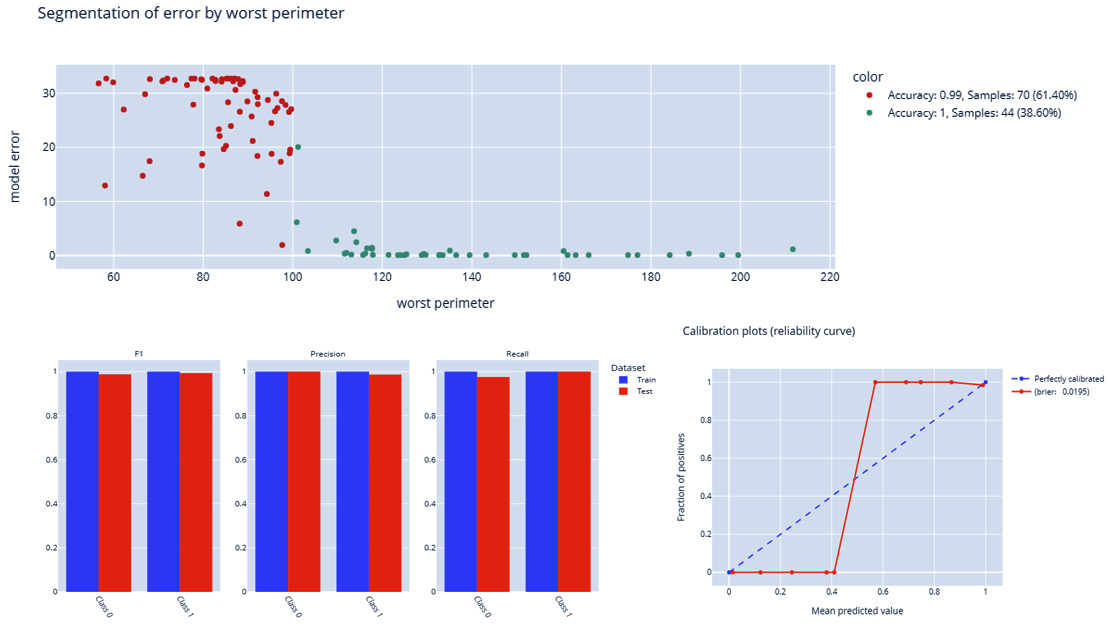
Figure 3.7 – Data forecastability using the model evaluation report and the Deepchecks framework

Next, let's discuss how to estimate data forecastability.

Estimating data forecastability

Data forecastability is estimated using the model evaluation metrics. Data forecastability can also be measured by performing model error analysis. The choice of the metrics depends on the type of dataset and the type of problem being solved. For example, take a look at the following list:

• For time series data, data forecastability is obtained by metrics such as the mean absolute percentage error (MAPE), the symmetric mean absolute percentage error (SMAPE), the coefficient of variation (CoV), and more.
• For classification problems, I usually go for ROC-AUC Scores, the confusion matrix, precision, recall, and F1 scores along with accuracy.
• For regression problems, we can look at the mean square error (MSE), the R2 score, the root mean square error (RMSE), the sum of squared errors (SSE), and more.

You might have already used most of these metrics to evaluate trained ML models. Data forecastability is not just about evaluating trained models according to your choice of metric, but is the measure of predictability of the model using the given dataset.

Let's suppose you are applying three different ML algorithms such as decision trees, support vector machine (SVM), and random forests for a classification problem, and your choice of metric is recall. This is because your goal is to minimize the impact of false positives. After rigorous training and validation on the unseen data, you are able to obtain recall scores of 70% with decision tree, 85% with SVM, and 90% with random forest. What do you think your data forecastability will be? Is it 70%, 90%, or 81.67% (the average of the three scores)?

I would say that the correct answer is between 70% and 90%. It is always better to consider forecastability as a ballpark estimate, as providing a range of values rather than a single value gives an idea of the best-case and worst-case scenarios. Communicating about the data forecastability increases the confidence of the end stakeholders in ML systems. If the end users are consciously aware that the algorithm is only 70% accurate, they will not blindly trust the model even if the system predicts incorrectly. The end users would be more considerate if the model outcome does not match the actual outcome when they are aware of the model's limitations.

Most ML systems in production have started using prediction probability or model confidence as a measure of data forecastability, which is communicated to the end users. For example, nowadays, most weather forecasting applications show that there is a certain percentage of chance (or probability) for rainfall or snowfall. Therefore, data forecastability increases the explainability of AI algorithms by setting up the right expectation for the accuracy of the predicted outcome. It is not just the measure of the model performance, but rather a measure of the predictability of a model which is trained on a specific dataset.

This brings us to the end of the chapter. Let's summarize what we have discussed in the following section.

Summary

Now, let's try to summarize what you have learned in this chapter. In this chapter, we focused on data-centric approaches for XAI. We learned the importance of explaining black-box models with respect to the underlying data, as data is the central part of any ML model. The concept of data-centric XAI might be new to many of you, but it is an important area of research for the entire AI community. Data-centric XAI can provide explainability to the black-box model in terms of data volume, data consistency, and data purity.

Data-centric explainability methods are still active research topics, and there is no single Python framework that exists that covers all of the various aspects of data-centric XAI. Please explore the supplementary Jupyter notebook tutorials provided at https://github.com/PacktPublishing/Applied-Machine-Learning-Explainability-Techniques/tree/main/Chapter03 to gain more practical knowledge on this topic.

We learned about the idea of thorough data inspection and data profiling to estimate the consistency of training data and inference data. Monitoring data drifts for production ML systems is also an essential part of the data-centric XAI process. Apart from data drifts, estimating the adversarial robustness of ML models and the detection of adversarial attacks form an important part of the process.

Finally, we learned about the importance of data forecastability to set the right expectation to end stakeholders about what the model can achieve and how this is a necessary practice that can increase the trust of our end users.

You have been introduced to many statistical concepts in this chapter. Covering everything about each statistical method is beyond the scope of this chapter. However, I strongly recommend that you go through the reference links shared to understand these topics in greater depth.

This brings us to the end of part 1 of this book, in which you have been exposed to the conceptual understanding of certain key topics of XAI. From the next chapter onward, we will start exploring popular Python frameworks for applying the concepts of XAI to practical real-world problems. In the next chapter, we will cover an important XAI framework called LIME and examine how it can be used in practice.

References

To gain additional information about the topics in this chapter, please refer to the following resources:

• Andrew Ng Launches A Campaign For Data-Centric AI: https://www.forbes.com/sites/gilpress/2021/06/16/andrew-ng-launches-a-campaign-for-data-centric-ai/?sh=5333db3a74f5
• Landing.AI: Data-Centric AI: https://landing.ai/data-centric-ai/
• Jiang et al. "To Trust Or Not To Trust A Classifier" (2018): https://arxiv.org/abs/1805.11783
• Deepchecks: https://docs.deepchecks.com/en/stable/
• Statistical distance: https://en.wikipedia.org/wiki/Statistical_distance
• Lin et al. "Examining Distributional Shifts by Using Population Stability Index (PSI) for Model Validation and Diagnosis": https://www.lexjansen.com/wuss/2017/47_Final_Paper_PDF.pdf
• Wasserstein metric: https://en.wikipedia.org/wiki/Wasserstein_metric
• Bhattacharyya Distance based Concept Drift Detection Method For evolving data stream: https://www.researchgate.net/publication/352044688_Bhattacharyya_Distance_based_Concept_Drift_Detection_Method_For_evolving_data_stream