Chapter 2: Model Explainability Methods

One of the key goals of this book is to empower its readers to design Explainable ML systems that can be used in production to solve critical business problems. For a robust Explainable ML system, explainability can be provided in multiple ways depending on the type of problem and the type of data used. Providing explainability for structured tabular data is relatively human-friendly compared to unstructured data such as images and text, as image or text data is more complex with less interpretable granular features.

There are different ways to add explainability to ML models, for instance, by extracting information about the data or the model (knowledge extraction), using effective visualizations to justify the prediction outcomes (result visualization), identifying dominant features in the training data and analyzing its effect on the model predictions (influence-based methods), or by comparing model outcomes with known scenarios or situations as an example (example-based methods).

So, in this chapter, we are going to discuss various model-agnostic and model-specific explanation methods that are used for both structured and unstructured data for model explainability.

This chapter covers the following main topics:

• Types of model explainability methods
• Knowledge extraction methods
• Result visualization methods
• Influence-based methods
• Example-based methods

Technical requirements

The primary goal of this chapter is to provide a conceptual understanding of the model explainability methods. However, I will provide certain tutorial examples to implement some of these methods in Python on certain interesting datasets. We will be using Python Jupyter notebooks to run the code and visualize the output throughout this book. The code and dataset resources for Chapter 2 can be downloaded or cloned from the following GitHub repository: https://github.com/PacktPublishing/Applied-Machine-Learning-Explainability-Techniques/tree/main/Chapter02. Other important Python frameworks that are required to run the code will be mentioned in the notebooks along with other relevant details to understand the code implementations within these concepts.

Types of model explainability methods

There are different approaches that you can use to provide model explainability. Certain techniques are specific to a model, and certain approaches are applied to the input and output of the model. In this section, we will discuss the different types of methods used to explain ML models:

• Knowledge extraction methods: Extracting key insights and statistical information from the data during Exploratory Data Analysis (EDA) and post-hoc analysis is one way of providing model-agnostic explainability. Often, statistical profiling methods are applied to extract the mean and median values, standard deviation, or variance across the different data points, and certain descriptive statistics are used to estimate the expected range of outcomes.

Similarly, other insights using correlation heatmaps, decomposition trees, and distribution plots are also used to observe any relationships between the features to explain the model's results. For more complex unstructured data, such as images, often, these statistical knowledge extraction methods are not sufficient. Human-friendly methods using Concept Activation Vectors (CAVs), as discussed in Chapter 8, Human-Friendly Explanations with TCAV, are more effective.

However, primarily, knowledge extraction methods extract essential information about the input data and the output data from which the expected model outcomes are defined. For example, to explain a time series forecasting model, we can consider a model performance metric such as the variance in forecasting error over the training period. The error rate can be specified within a confidence interval of (let's say) +/- 10%. The formation of the confidence interval is only possible after extracting key insights from the output training data.

• Result visualization methods: Plotting model outcomes and comparing them with previously predicted values, particularly with surrogate models, is often considered an effective model-agnostic explainability method. Predictions from black-box ML algorithms are passed to the surrogate model explainers. Usually, these are highly interpretable linear models, decision trees, or any rule-based heuristic algorithm that can explain the outcome of complex models. The main limitation of this approach is that the explainability is solely dependent on the model outcome. If there is any abnormality with the data or the modeling process, such dimensions of explainability are not captured.

For example, let's suppose a classifier is incorrectly predicting an output. It is not feasible for us to understand exactly why the model is behaving in a specific manner just from the prediction probability. But these methods are easy to apply in practice and even easy to understand as highly interpretable explainer algorithms are used.

• Influence-based methods: These are specific techniques that help us to understand how certain data features play an important role in influencing or controlling the model outcome. Right now, this is one of the most common and effective methods applied to provide explainability to ML models. Feature importance, sensitivity analysis, key influencer maps, saliency maps, Class Activation Maps (CAMs), and other visual feature maps are used to interpret how the individual features within the data are being utilized by the model for its decision-making process.
• Example-based methods: The three previously discussed model-agnostic explainability methods still need some kind of technical knowledge to understand the working of the ML models. For non-technical users, the best way to explain something is to provide an example that they can relate to. Example-based methods, particularly counterfactual example-based methods, try to look at certain single instances of the data to explain the ML models' decision-making process.

For example, let's say an automated loan approval system powered by ML denies a loan request to an applicant. Using example-based explainability methods, the applicant will also be suggested that if they pay their credit card bill on time for the next three months and increase their monthly income by $2,000, their loan request would be granted.

Based on the latest trends, model-agnostic techniques are preferred over model-dependent approaches as even complex ML algorithms can be explained, to some degree, using these techniques. But certain techniques such as saliency maps, tree/forest-based feature importance, and activation maps are mostly model-specific. Our choice of explanation method is determined by the key problem that we are trying to solve.

Figure 2.1 illustrates the four main types of explainability methods that have been applied to explain the working of black-box models, which we are going to cover in the following sections:

Figure 2.1 – Model explainability methods

Now, let's start by discussing each of these model explainability methods in more detail.

Knowledge extraction methods

Whenever we talk about explainability in any context, it is all about gaining knowledge of the problem so as to gain some clarity about the expected outcome. Similarly, if we already know the outcome, explainability is all about tracing back to the root cause. Knowledge extraction methods in ML are used to extract key insights from the input data or utilize the model outcome to trace back and map to certain information known to the end users for both structured data and unstructured data. Although there are multiple approaches to extracting knowledge, in practice, the data-centric process of EDA is one of the most common and popular methods for explaining any black-box model. Let's discuss more on how to use the EDA process in the context of XAI.

EDA

I would always argue that EDA is the most important process for any ML workflow. EDA allows us to explore the data and draw key insights; using this, we can form certain hypotheses from the data. This actually helps us to identify any distinct patterns within the data and will, eventually, help us to make the right choice of algorithm. Thus, EDA is one of the conventional and model-agnostic approaches that explain the nature of the data, and by considering the data, it helps us understand what to expect from the model. Detecting any clear anomaly, ambiguous, redundant data points and bias in data can be easily observed using EDA. Now, let's see some important methods used in EDA to explain ML models for structured and unstructured data.

EDA on structured data

EDA on structured data is one of the preliminary steps applied for extracting insights to provide explainability. However, the actual techniques applied in the EDA process could vary from one problem to another. But generally, for structured data, we can use EDA to generate certain descriptive statistics for a better understanding of the data and then apply various univariate and multivariate methods to detect the importance of each feature, observe the distribution of data to find any biases in the data, and look for outliers, duplicate values, missing values, correlation, and cardinality between the features, which might impact the model's results.

Information and hypotheses obtained from the EDA step help perform meaningful feature engineering and modeling techniques and help set up the right expectation for the stakeholders. In this section, we will cover the most popular EDA methods and discuss the benefit of using EDA with structured data in the context of XAI. I strongly recommend looking at the GitHub repository (https://github.com/PacktPublishing/Applied-Machine-Learning-Explainability-Techniques) to apply some of these techniques in practice for practical use cases. Now, let's look at the important EDA methods in the following list:

• Summary statistics: Usually, model explainability is presented with respect to the features in the data. Observing dataset statistics during the EDA process gives an early indication of whether the dataset is sufficient for modeling and solving the given problem. It helps to understand the dimensions of the data and the type of features present. If the features are numeric, certain descriptive statistics such as the mean, standard deviation, coefficient of variation, skewness, kurtosis, and inter-quartile ranges are observed.

Additionally, certain histogram-based distributions are used to monitor any skewness or biases in data. For categorical features, the frequency distribution of the categorical values is observed. If the dataset is imbalanced, if the dataset is biased toward a particular categorical value, if the dataset has outliers, or is skewed toward a particular direction, all of these can be easily observed. Since all of these factors can impact the model predictions, understanding dataset statistics is important for model explainability.

Figure 2.2 shows the summary statistics and visualizations created during the EDA step to extract knowledge about the data:

Figure 2.2 – Summary statistics and visualizations during EDA

• Duplicate and missing values: Duplicate or redundant values can add more bias to the model. In contrast, missing values can lead to a loss of information and insufficient data to train the model. This might lead to model-overfitting. So, before training the model, if missing values or duplicate values are observed, and if further actions are not taken to rectify this, then these observations might help to explain the reason behind the non-generalization of models.
• Univariate analysis: This involves analyzing a single feature through graphical techniques such as distribution plots, histograms, box plots, violin plots, pie charts, clustering plots, and using non-graphical techniques such as frequency, central tendency measures (that is, the mean, standard deviation, and coefficient of variation), and interquartile ranges. These methods help us to estimate the impact of individual features on the model outcome.
• Multivariate analysis: This involves analyzing two or more features together using graphical and non-graphical methods. It is used for identifying data correlation and the dependencies of variables. In the context of XAI, multivariate analysis is used to understand complex relationships in the data and provide a detailed and granular explanation as compared to univariate analysis methods.
• Outlier detection: Outliers are certain abnormal data points that can completely skew the model. It is hard to achieve generalization if a model is trained on outlier data points. However, model prediction can go completely wrong during the model inference time for an anomaly datapoint. Hence, outlier detection during both training and inference time is an important part of model explainability. Visualization methods such as box plots, scatter plots, and statistical methods such as the 1.5xIQR rule (https://www.khanacademy.org/math/statistics-probability/summarizing-quantitative-data/box-whisker-plots/a/identifying-outliers-iqr-rule) and Nelson's Rule (https://www.leansixsigmadefinition.com/glossary/nelson-rules/) are used for detecting anomalies.
• Pareto analysis: According to the Pareto Principle, 80% of the value or impact is driven by 20% of the sample size. So, in XAI, this 80–20 rule is used to interpret the most impactful sub-samples that have the maximum impact on the model outcome.
• Frequent Itemset Mining: This is another popular choice of approach to extract model explainability. This technique is used frequently for Association rule mining to understand how frequently certain observations occur together in any given dataset. This method provides some interesting observations that help to form important hypotheses from the data and, eventually, contribute a lot to explaining model outcomes.

Now that we have covered the methods for structured data, let's take a look at some of the methods for unstructured data.

EDA on unstructured data

Interpreting features from unstructured data such as images and text is difficult, as ML algorithms try to identify granular-level features that are not intuitively explainable to human beings. Yet, there are certain specific methods applied to image and text data to form meaningful hypotheses from the data. As discussed earlier, the EDA process might change based on the problem and the data, but in this chapter, we will discuss the most popular choice of methods in the context of XAI.

Exploring image data

EDA methods used for images are different from the methods used with tabular data. These are some popular choices of EDA steps for image datasets:

• Data dimension analysis: For consistent and generalized models, understanding data dimension is important. Monitoring the number of images and the shape of each image is important to explain any observation of overfitting or underfitting.
• Observing data distribution: Since the majority of problems solved using images are classification problems, monitoring class imbalance is important. If the distribution of data is not balanced, then the model can be biased toward the majority class. For pixel-level classification (for segmentation problems), observing pixel intensity distribution is important. This also helps in understanding the effect of shadow or non-uniform lighting conditions on images.
• Observing average images and contrast images: For observing dominant regions of interest in images, average and contrast images are often used. This is especially used for classification-based problems to compare dominant regions of interest.
• Advanced statistical and algebraic methods: Apart from the methods discussed so far, other statistical methods such as finding the z-score and standard deviation, and algebraic methods such as Eigenimages based on eigenvectors are used to visually inspect key features in image data, which adds explainability to the final model outcome.

There are other complex methods to explore image datasets depending on the type of the problem. However, the methods discussed in this subsection are the most common approaches.

Exploring text data

Usually, text data is noisier in comparison to images or tabular datasets. Hence, EDA is usually accompanied by some preprocessing or cleaning methods for text data. But since we are focusing only on the EDA part, the following list details some of the popular approaches to do EDA with text data:

• Data dimension analysis: Similar to images, text dimension analyses, such as checking the number of records and the length of each record, are performed to form hypotheses about potential overfitting or underfitting.
• Observing data distribution: Visualizing the distribution of word frequency using bar plots or word clouds are popular choices in which to observe top words in any text data. This technique allows us to avoid any bias of high-frequency words as compared to low-frequency words.
• n-gram analysis: Considering the nature of text data, often, a phrase or collection of words is more interpretable than only a single word. For example, for sentiment analysis from movie reviews, individual words with a high frequency such as movie or film are quite ambiguous. In contrast, phrases such as good movie and very boring film are far more interpretable and useful to understand the sentiments. Hence, n-gram analysis or taking a collection of "n-words" brings more explainability for understanding the model outcome.

Usually, EDA does include certain visualization techniques to explain and form some important hypotheses from the data. But another important technique to explain ML models is by visualizing the model outcome. In the next section, we will discuss these result visualization methods in more detail.

Result visualization methods

Visualization of the model outcomes is a very common approach applied to interpret ML models. Generally, these are model-agnostic, post-hoc analysis methods applied on trained black-box models and provide explainability. In the following section, we will discuss some of the commonly used result visualization methods for explaining ML models.

Using comparison analysis

These are mostly post-hoc analysis methods that are used to add model explainability by visualizing the model's predicted output after the training process. Mostly, these are model-agnostic approaches that can be applied to both intrinsically interpretable models and black-box models. Comparison analysis can be used to produce both global and local explanations. It is mainly used to compare different possibilities of outcomes using various visualization methods.

For example, for classification-based problems, certain methods such as t-SNE and PCA are used to visualize and compare the transformed feature spaces of the model predicted labels, especially when the error rate is high. For regression and time series predictive models, confidence levels are used to compare model predicted results with the upper and lower bounds. There are various methods to apply comparison analysis and get a clearer idea of the what-if scenarios. Some prominent methods are mentioned in the project repository (https://github.com/PacktPublishing/Applied-Machine-Learning-Explainability-Techniques/blob/main/Chapter02/Comparison%20Analysis.ipynb).

As we can see in Figure 2.3, result visualization can help to provide a global perspective about the model to visualize model predictions:

Figure 2.3 – Comparison analysis using the t-SNE method for the classification problem (left-hand side) and the time series prediction model with the confidence interval (right-hand side)

In Figure 2.3, we can see how visualization methods can be used to provide local explanations by visualizing the final outcome of the model and comparing the outcome with either other data instances or with possible what-if scenarios to provide a global perspective of the model.

Using Surrogate Explainer methods

In the context of ML, when an external model or algorithm is applied to interpret a black-box ML model, the external method is known as the Surrogate Explainer method. The fundamental idea behind this approach is to apply an intrinsically explainable model that is simple and easy to interpret and approximate the predictions of the black-box model as accurately as possible. Then, certain visualization techniques are used to visualize the outcome from the Surrogate Explainer methods to get insights into the model behavior.

But now the question is can we apply surrogate models directly instead of using the black-box model? The answer is no! The main idea behind using the surrogate model is to get some information about how the input data is related to the target outcomes, without considering the model accuracy. In contrast, the original black-box model is more accurate and efficient but not interpretable. So, replacing the black-box model completely with the surrogate model would compromise the model accuracy, which we don't want.

Interpretable algorithms such as regression, decision trees, and rule-based algorithms are popular choices for Surrogate Explainer methods. To provide explainability, mainly three types of relationships between the input features and the target outcome are analyzed: linearity, monotonicity, and interaction.

Linearity helps us to inspect whether the input features are linearly related to the target outcome. Monotonicity helps us to analyze whether increasing the overall input feature values leads to either an increase or a decrease in the target outcome. For the entire range of features, this explains whether the relationship between the input features and the target always propagates in the same direction. Model interactions are extremely helpful when providing explainability, but it is tough to achieve. Interactions help us to analyze how individual features interact with each other to impact the model decision-making process.

Decision trees and rule-based algorithms are used to inspect interactions between the input features and the target outcome. Christoph Molner, in his book Interpretable Machine Learning (https://christophm.github.io/interpretable-ml-book/), has provided a very useful table comparing different intrinsically interpretable models, which can be useful for selecting interpretable models as a Surrogate Explainer model.

A simplified version of this is shown in the following table:

Figure 2.4 – Comparing interpretable algorithms for selecting a Surrogate Explainer method

One of the major advantages of this technique is that it can help to make any black-box model interpretable. It is model-agnostic and very easy to implement. But when the data is complex, more sophisticated algorithms are used to achieve higher modeling accuracy. In such cases, surrogate methods tend to oversimplify complicated patterns or relationships between the input features.

Figure 2.5 illustrates how interpretable algorithms such as decision trees, linear regression, or any heuristic rule-based algorithm can be used as surrogate models to explain any black-box ML model:

Figure 2.5 – Using Surrogate explainers for model explainability

Despite the drawbacks of this approach, visualization of linearity, monotonicity, and interaction can justify working on complex black-box models to a great extent. In the next section, we will discuss influence-based methods to explain ML models.

Influence-based methods

Influence-based methods are used to understand the impact of features present in the dataset on the model's decision-making process. Influence-based methods are widely used and preferred in comparison to other methods as this helps to identify the dominating attributes from the dataset. Identifying the dominating attributes from structured and unstructured data helps us analyze the dominating features' role in influencing the model outcome.

For example, let's say you are working on a classification problem for classifying wolves and Siberian huskies. Let's suppose that after the training and evaluation process, you have achieved a good model with more than 95% accuracy. But when trying to find the important features using influence-based methods for model explainability, you observed that the model picked up the surrounding background as the dominating feature to classify whether it is a wolf or a husky. In such cases, even if your model result seems to be highly accurate, your model is unreliable. This is because the features that the model was making the decision on are not robust and generalized.

Influence-based methods are popularly used for performing root cause analysis to debug ML models and detect failures in ML systems. Now, let's discuss some of the popular choices of the influence-based methods that are used for model explainability.

Feature importance

When applying an ML model, understanding the relative importance of each feature in terms of influencing the model outcome is crucial. It is a technique that assigns a particular score to the input features present in the dataset based on the usefulness of the features in predicting the target value. Feature importance is a very popular choice of model-agnostic explainability for modeling structured data. Although there are various scoring mechanisms to determine feature importance, such as permutation importance scores, statistical correlation scores, decision tree-based scoring, and more, in this section, we will mostly focus on the overall method and not just on the scoring mechanism.

In the context of XAI, feature importance can provide global insights into the data and the model behavior. It is often used for feature selection and dimensionality reduction to improve the efficiency of ML models. By removing less important features from the modeling process, it has been observed that, usually, the overall model performance is improved.

The notion of important features can sometimes depend on the type of scoring mechanism or the type of model used. So, it is recommended that you validate the important features picked up by this technique with domain experts before drawing any conclusions. This method is applied to structured datasets, where the features are clearly defined. For unstructured data such as text or images, feature importance is not very relevant as the features or patterns used by the model are more complex and not always human interpretable.

Figure 2.6 illustrates how highlighting the influential features of a dataset enables the end user to focus on the values of the important features to justify the model outcome:

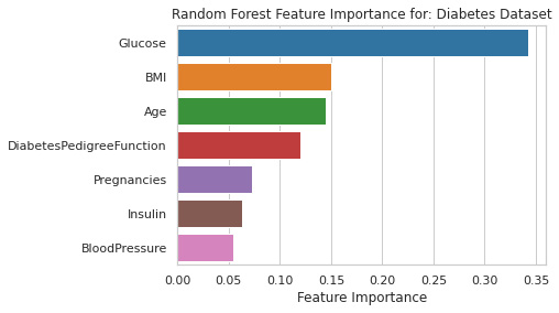
Figure 2.6 – A feature importance graph on the diabetes dataset (from the code tutorials)

Next, we will cover another important influence-based model explainability method, called sensitivity analysis.

Sensitivity analysis

Sensitivity analysis is a quantitative process that approximates uncertainty in forecasts by altering the assumptions made about important input features used by the forecasting model. In sensitivity analysis, the individual input feature variables are increased or decreased to assess the impact of the individual features on the target outcome. This technique is very commonly used in predictive modeling to optimize the overall performance and robustness of the system.

Conducting sensitivity analysis can be simple yet a very powerful method for any data science project, which can provide additional information to business stakeholders, especially for multivariate datasets. It helps to understand the what-if scenarios and observe whether any particular feature is sensitive to outliers or any form of adversarial perturbations. It helps in questioning the reliability of variable assumptions, can predict the possible outcomes if the assumptions are changed, and can measure the significance of altering variable assumptions. Sensitivity analysis is a data-driven modeling approach. It indicates whether the data is reliable, accurate, and relevant for the modeling process. Additionally, it helps to find out whether there are other intervening factors that can impact the model.

In the context of XAI, since sensitivity analysis is slightly less common as compared to some of the widely used methods, let me try to give my recommendations for performing sensitivity analysis in ML. Usually, this is very useful for regression problems, but it is quite important for classification-based problems, too.

Please refer to the notebook (https://github.com/PacktPublishing/Applied-Machine-Learning-Explainability-Techniques/blob/main/Chapter02/FeatureImportance_SensitivityAnalysis.ipynb) provided in the GitHub repository to get a detailed and practical approach for doing sensitivity analysis. The very first step that I recommend you do for sensitivity analysis is to calculate the standard deviation (σ) of each attribute that is present in the raw dataset. Then, for each attribute, transform the original attribute values to -3σ, -2σ, -σ, σ, 2σ, and 3σ, and either observe and plot the percentage change in the target outcome for a regression problem or observe the predicted class for a classification-based problem.

For a good and robust model, we would want the target outcome to be less sensitive to any change in the feature values. Ideally, we would expect the percentage change in the target outcome to be less drastic for regression problems, and for classification problems, the predicted class should not change much on changing the feature values. Any feature value beyond +/- 3σ is considered an outlier, so usually, we vary the feature values up to +/- 3σ.

Figure 2.7 shows how detailed sensitivity analysis helps you analyze factors that can easily influence the model outcome:

Figure 2.7 – Sensitivity analysis to understand the influential features of the data

Apart from sensitivity analysis, in the next section, you will learn about Partial Dependence Plots (PDPs), which can also be used to analyze influential features.

PDPs

When using black-box ML models, inspecting functional relations between feature attributes and target outcomes can be challenging. Although calculating feature importance can be easier, PDPs provide a mechanism to functionally calculate the relationship between the predictive features and the predictor variables. It shows the marginal effect one or two attributes have on the target outcome.

PDPs can effectively help pick up linear, monotonic, or any complex interaction between the predictive variables and the predictor variables and indicate the overall impact that the predictor variable has on the predictive variable on average. PDP includes the contribution of particular predictor attributes by measuring the marginal effect, which does not include the other variables' impact on the feature space.

Similar to sensitivity analysis, PDPs help us to approximate the direction in which specific features can influence the target outcome. For the sake of simplicity, I will not add any complex mathematical representation of partial dependence to obtain the average marginal effect of predictor variables; however, I would strongly recommend going through Jerome H. Friedman's work on Greedy Function Approximation: A Gradient Boosting Machine to get more information. One of the most significant benefits of PDP is that it is straightforward to use, implement, and understand and can be explained to a non-technical business stakeholder or an end user of ML models very easily.

But there are certain drawbacks to this approach, too. By default, the approach assumes that all features are not correlated and there is no interaction between the feature attributes. In any practical scenario, this is highly unlikely to happen, as the majority of the time, there will be some interaction or joint effect due to the feature variables.

PDPs are also limited to two-dimensional representations, and PDPs do not show any feature distribution. So, if the feature space is not evenly distributed, certain effects of bias can get missed while analyzing the outcome. PDPs might not show any heterogeneous effects as it only shows the average marginal effects. This means that if half of the data for a particular feature has a positive impact on the predicted outcome, and the other half has a negative effect on the predicted outcome, then the PDP could just be a horizontal line as the effects from both halves can cancel each other. This can lead to the conclusion that the feature does not have any impact on the target variable, which is misleading.

The drawbacks of PDP can be solved by Accumulated Local Effect Plots (ALEP) and Individual Conditional Expectation Curves (ICE curves). We will not be covering these concepts in this chapter, but please refer to the Reference section, [Reference – 4,5], to get additional resources to help you understand these concepts.

Let's look at some sample PDP visualizations from Figure 2.8:

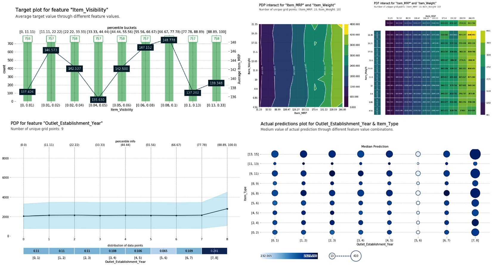
Figure 2.8 – PDP visualizations (from the code tutorial)

Figure 2.8 illustrates PDP visualizations that help us to understand influential features from tabular datasets. In the next section, we will discuss the Layer-wise Relevance Propagation (LRP) methods to understand influential features from unstructured data.

LRP

Most of the influence-based methods that we discussed earlier are highly effective for structured data. But unfortunately, these methods cannot be applied to unstructured data such as images and texts where the features are not always clearly defined, especially when using Deep Convolution Neural Networks (DCNNs). Classical ML algorithms are not efficient as compared to deep learning algorithms when applied to unstructured data such as images and text. Due to the benefit of automatic feature extraction in deep learning as compared to manual feature engineering in classical ML, deep learning algorithms are more efficient in terms of model accuracy and, hence, more preferred. However, deep learning models are more complex and less interpretable than classical ML models.

Providing explainability to deep learning models is also quite challenging; usually, there are very few quantitative ways for providing explainability to deep learning models. Therefore, we mostly rely on qualitative approaches to visualize the key influencing data elements that can impact the process of calculating weights and biases, which are the main parameters of any deep learning model. Moreover, for deep networks with multiple layers, learning happens when the flow of information through the gradient flow process between the layers is maintained consistently. So, to explain any deep learning model, particularly for images and text, we would try to visualize the activated or most influential data elements throughout the different layers of the network and qualitatively inspect the functioning of the algorithm.

To explain deep learning models, LRP is one of the most prominent approaches. Intuitively speaking, this method utilizes the weights in the network and the forward pass neural activations to propagate the output back to the input layer through the various layers in the network. So, with the help of the network weights, we can visualize the data elements (pixels in the case of images and words in the case of text data) that contributed most toward the final model output. The contribution of these data elements is a qualitative measure of relevance that gets propagated throughout the network layers.

Now, we will explore some specific LRP methods that have been applied to explain the working of deep learning models. In practice, implementing these methods can be challenging. So, I have not included these methods in the code tutorials, as this chapter is supposed to help even beginner learners. I have shared some resources in the Reference section for intermediate or advanced learners for the code walk-throughs.

Saliency maps

A saliency map is one of the most popularly used approaches for interpreting the prediction of Convolution Neural Networks (CNNs). This technique is derived from the concept of image saliency, which refers to the important features of an image, such as the pixels, which are visually alluring. So, a saliency map is another image derived from the original image in which the pixel brightness is directly proportional to the saliency of the image. A saliency map helps to highlight regions within the image that play an important role in the final decision-making process for the model. It is a visualization technique used specifically in DCNN models to differentiate visual features from the data.

Apart from providing explainability to deep learning models, saliency maps can be used to identify regions of interest, which can be further used by automated image annotation algorithms. Also, saliency maps are used in the audio domain, particularly in audio surveillance, to detect unusual sound patterns such as gunshots or explosions.

Figure 2.9 shows the saliency map for a given input image, which highlights the important pixels used by the model to predict the outcome:

Figure 2.9 – Saliency maps for an input image

Next, let's cover another popular LRP method – Guided Backpropagation (Guided Backprop).

Guided backprop

Another visualization technique used for explaining deep learning models to increase trust and their adoption is guided backprop. Guided backprop highlights granular visual details in an image to interpret why a particular class was predicted by the model. It is also known as guided saliency and actually combines the process of vanilla backpropagation and backpropagation through ReLU nonlinearity (also referred to as DeconvNets). I would strongly recommend looking at this article, https://towardsdatascience.com/review-deconvnet-unpooling-layer-semantic-segmentation-55cf8a6e380e, to learn more about the backpropagation and the DeconvNet mechanism if you are not aware of these terms.

In this method, the neurons of the network act as the feature detectors and, because of the usage of the ReLU activation function, only gradient elements that are positive in the feature map are kept. Additionally, the DeconvNets only keep the positive error signals. Since the negative gradients are set to zero, only the important pixels are highlighted when backpropagating through the ReLU layers. Therefore, this method helps to visualize the key regions of the image, the vital shapes, and the contours of the object that are to be classified by the algorithm.

Figure 2.10 shows a guided backprop map for a given input image that marks the contours and some granular visual features used by the model to predict the outcome:

Figure 2.10 – Guided backprop for an input image

Guided backprop is very useful, but in the next section, we will cover another useful method to explain unstructured data such as images, called the Gradient CAM.

Gradient CAM

CAMs are separate visualization methods used for explaining deep learning models. Here, the model predicted class scores are traced back to the last convolution layer to highlight discriminative regions of interest in the image that are class-specific and not even generic to other computer vision or image processing algorithms. Gradient CAM combines the effect of guided backprop and CAM to highlight class discriminative regions of interest without highlighting the granular pixel importance, unlike guided backprop. But Grad-CAM can be applied to any CNN architectures, unlike CAM, which can be applied to architectures that perform global average pooling over output feature maps coming from the convolution layer, just prior to the prediction layer.

Grad-CAM (also referred to as Gradient-Weighted Class Activation Map) helps to visualize high-resolution details, which are often superimposed on the original image to highlight dominating image regions for predicting a particular class. It is extremely useful for multi-class classification models. Grad-CAM works by inspecting the gradient information flow into the last layer of the model. However, for certain cases, it is important to inspect fine-grained pixel activation information, too. Since Grad-CAM doesn't allow us to inspect granular information, there is another variant of Grad-CAM, which is known as Guided Grad-CAM, used to combine the benefits of guided backprop with Grad-CAM to even visualize the granular-level class discriminative information in the image.

Figure 2.11 shows what a Grad-CAM visualization looks like for any input image:

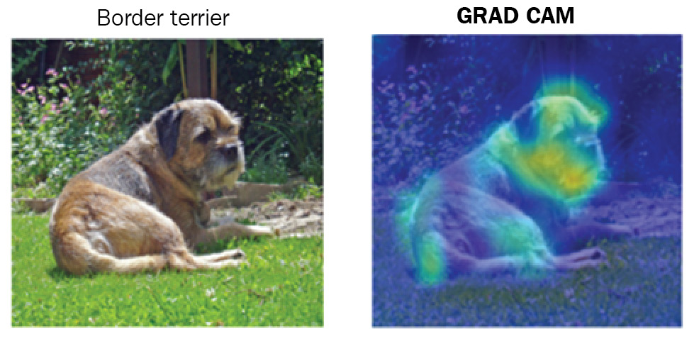
Figure 2.11 – Grad-CAM for an input image

Grad-CAM highlights the important regions in the image, which are used by the model to predict the outcome. Another variant of this approach is to use guided Grad-CAM, which combines the guided backpropagation and Grad-CAM methods to produce interesting visualizations to explain deep learning models:

Figure 2.12 – Architecture diagram for guided Grad-CAM

Figure 2.12 shows the architecture diagram for the guided Grad-CAM approach that is slightly more complex to understand. But overall, LRP is an important approach that can be used to explain the functioning of deep learning models.

Representation-based explanation

Pattern representation plays an important role in the decision-making process, especially for unstructured data such as text and images. Conventionally, hand-engineered pattern matching algorithms were used for extracting global features, which human beings can relate to. But recently, GoogleAI's model interpretability technique, which is based on CAVs, gained great popularity in the field of XAI. In this part, we will discuss CAVs in more detail, although extracting features and patterns from unstructured data also falls under the representation-based explanations.

CAVs

Particularly for unstructured data, most deep learning models work on low-level features such as edges, contours, and motifs, and some mid-level and high-level features such as certain defined parts and portions of the object of interest. Most of the time, these representations are not human-friendly, especially for complex deep learning models. Intuitively, CAVs relate the presence of low-level and granular features to high-level human-friendly concepts. Therefore, model explainability with CAVs provides more realistic explanations to which any human being can relate.

The approach of CAVs is actually implemented using the Testing with Concept Activation Vectors (TCAV) framework from GoogleAI. TCAV utilizes directional derivatives to approximate the internal state of the neural network to a human-defined concept. For example, if we ask a human being to explain what a zebra looks like, they would probably say that a zebra is an animal that looks like a white horse with black stripes and is found in grasslands. So, the terms animal, white horse, black stripes, and grasslands can be important concepts used to represent zebras.

Similarly, the TCAV algorithm tries to learn these concepts and learn how much of the concept was important for the prediction using the trained model, although these concepts might not be used during the training process. So, TCAV tries to quantify how sensitive the model is toward the particular concept for a particular class. I found the idea of CAVs very appealing. I think it is a step toward creating human-friendly explanations of AI models, which any non-technical user can easily relate to. We will be discussing the TCAV framework from GoogleAI, in more detail, in Chapter 8, Human-Friendly Explanations with TCAV.

Figure 2.13 illustrates the idea of using human-friendly concepts to explain model predictions. In the next subsection, we will see another visualization approach that is used to explain complex deep learning models:

Figure 2.13 – The fundamental idea behind the CAV

Next, we will discuss Visual Attention Maps (VAMs), which can also be used with complicated deep learning models.

VAMs

In recent years, transformer model architectures have gained a lot of popularity because of their ability to achieve state-of-the-art model performance on complicated unstructured data. Attention networks are the heart of transformer architecture, which allows the algorithm to learn more contextual information for producing more accurate outcomes.

The basic idea is that every portion of the data is not equally important and only the important features need more attention than the rest of the data. Therefore, the attention network filters out irrelevant portions of the data for making a better judgment. By the attention mechanism, the network can assign higher weights to the important sections by the level of importance to the underlying task. Using these attention weights, certain visualizations can be created which explain the decision-making process of the complex algorithm. These are called VAMs.

This technique is particularly useful for Multimodal Encoder-Decoder architectures for solving problems such as automated image captioning and visual question answering. Applying VAMs can be quite complicated if you have a beginner level of understanding. So, I will not cover this technique in much detail in this book or in the code tutorials. If you are interested in learning more about how this technique work in practice, please refer to the code repository at https://github.com/sgrvinod/a-PyTorch-Tutorial-to-Image-Captioning.

As we can see in Figure 2.14, VAMs provide step-by-step visuals to explain the output of complex encoder-decoder models. In the next section, we will explore example-based methods, which are used to explain ML models:

Figure 2.14 – Using VAMs to explain complex encoder-decoder attention-based deep learning models for the task of automated image captioning using a multi-modal dataset

In the next section, we will cover another type of explainability method that uses human-friendly examples to interpret predictions from black-box models.

Example-based methods

Another approach to model explainability is provided by example-based methods. The idea of example-based methods is similar to how humans try to explain a new concept. As human beings, when we try to explain or introduce something new to someone else, often, we try to make use of examples that our audience can relate to. Similarly, example-based methods, in the context of XAI, try to select certain instances of the dataset to explain the behavior of the model. It assumes that observing similarities between the current instance of the data with a historic observation can be used to explain black-box models.

These are mostly model-agnostic approaches that can be applied to both structured and unstructured data. If the structured data is high-dimensional, it becomes slightly challenging for these approaches, and all the features cannot be included to explain the model. So, it works well only if there is an option to summarize the data instance or pick up only selected features.

In this chapter, we will mainly discuss Counterfactual Explanations (CFEs), the most popular example-based explainability method that works for both structured and unstructured data. CFEs indicate to what extent a particular feature has to change to significantly change the predicted outcome. Typically, this is useful for classification-based problems.

For certain predictive models, CFEs can provide prescriptive insights and recommendations that can be very crucial for end users and business stakeholders. For example, let's suppose there is an ML model used in an automated loan approval system. If the black-box model denies the loan request for a particular applicant, the loan applicant might reach out to the provider to learn the exact reason why their request was not approved. But instead, if the system suggests the applicant increases their salary by 5,000 and pay their credit card bills on time for the next 3 months in order to approve the loan request, then the applicant will understand and trust the decision-making process of the system and can work toward getting their loan request approved.

CFEs in structured data

Using the Diverse Counterfactual Explanation (DiCE) framework in Python (https://interpret.ml/DiCE/), a CFE can be provided for structured data. It can be applied to both classification and regression-based problems for model-agnostic local explainability, and it describes how the smallest change in the structured data can change the target outcome.

Another important framework used for CFEs in Python is Alibi (https://docs.seldon.io/projects/alibi/en/stable/), which is also pretty good in terms of implementing the concepts of CFE to explain ML models. Although we will be discussing these frameworks and experiencing the practical aspects of these frameworks in Chapter 9, Other Popular XAI Frameworks, for now, I will discuss some intuitive understanding of CFE on structured data. Please refer to the notebook (https://github.com/PacktPublishing/Applied-Machine-Learning-Explainability-Techniques/blob/main/Chapter02/Counterfactual_structured_data.ipynb) provided in the code repository to learn how to code these approaches in Python for practical problem-solving.

When used with structured data, the CFE method tries to analyze an input query data instance and tries to observe the original target outcome considering the same query instance from the historical data. Alternatively, it tries to inspect the features and maps them to a similar instance present in the historical data to get the target output. Then, the algorithm generates multiple counterfactual examples to predict the opposite outcome.

For a classification-based problem, this method would try to predict the opposite class for a binary classification problem or the nearest or most similar class for a multiclass classification problem. For a regression problem, if the target outcome is present toward the lower end of the spectrum, the algorithm tries to provide a counterfactual example with a target outcome closer to the higher end of the spectrum, and vice versa. Hence, this method is very effective for understanding what-if scenarios and can provide actionable insights along with model explainability. The explanations are also very clear and very easy to interpret and implement.

But the major drawback of this approach, particularly for structured data, is that it suffers from the Rashomon effect (https://www.dictionary.com/e/pop-culture/the-rashomon-effect/). For any real-world problem, it can find multiple CFEs that can contradict each other. With structured data, with multiple features, contradictory CFEs can create more confusion rather than explaining ML models! Human intervention and the application of domain knowledge to pick up the most relevant example can help in mitigating the Rashomon effect. Otherwise, my recommendation is to combine this method along with the feature importance method for actionable features to select counterfactual examples involving significant changes for providing better actionable explainability.

Figure 2.15 illustrates how CFEs can be used to get prescriptive insights and actionable recommendations to explain the working of models:

Figure 2.15 – Prescriptive insights obtained from CFEs in structured data

CFEs in tabular datasets can be very useful as they can provide actionable suggestions to the end user. In the next subsection, we will explore CFEs in unstructured data.

CFEs in unstructured data

In unstructured data such as images and text, implementing CFEs can be quite challenging. One of the main reasons for this is that the granular features used in images or text by deep learning models are not always well-defined or human-friendly. But the Alibi (https://docs.seldon.io/projects/alibi/en/stable/) framework does pretty well in generating CFEs on image data. Even the improved version of the simple CFE method performs even better by generating a CFE guided by class prototypes. It uses an auto-encoder or k-d trees to build a prototype for each prediction class using a certain input instance.

For example, in the MNIST dataset, let's suppose that the input query image is for digit 7. Then, the counterfactual prototype method will build prototypes of all the digits from 0 to 9. Following this, it will try to produce the nearest digit other than the original digit of 7 as the counterfactual example. Depending upon the data, the nearest hand-written digit can be either 9 or 1; even as human beings, we might confuse the digits 7 and 9 or 7 and 1 if the handwriting is not clear! It takes an optimization approach to minimize the model's counterfactual prediction loss.

I strongly recommend looking at Arnaud Van Looveren and Janis Klaise's work, Interpretable Counterfactual Explanations Guided by Prototypes (https://arxiv.org/abs/1907.02584), to get more details on how this approach works. This CFE method, guided by prototypes, also eliminates any computational constraint that can arise due to the numerical gradient evaluation process for black-box deep learning models. Please take a look at the notebook (https://github.com/PacktPublishing/Applied-Machine-Learning-Explainability-Techniques/blob/main/Chapter02/Counterfactual_unstructured_data.ipynb) in the GitHub repository to learn how to implement this method for practical problems.

The following diagram, which has been taken from the paper Counterfactual Visual Explanations, Goyal et al. 2019 (https://arxiv.org/pdf/1904.07451.pdf), shows how visual CFEs can be an effective approach for explaining image classifiers:

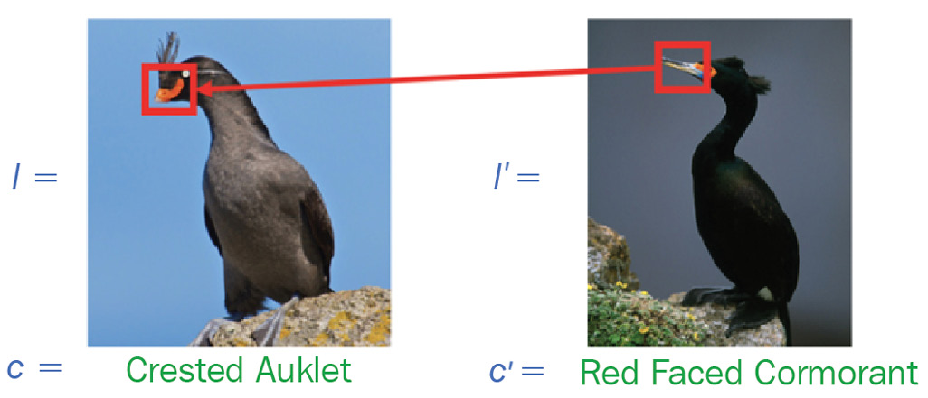
Figure 2.16 – A counterfactual example-based explanation for images

In practice, a CFE with unstructured data is difficult to achieve. It is still an area of active research, but I think this approach holds great potential to provide human-friendly explanations to even complex models. The following diagram shows the mapping of the various methods based on their explainability type:

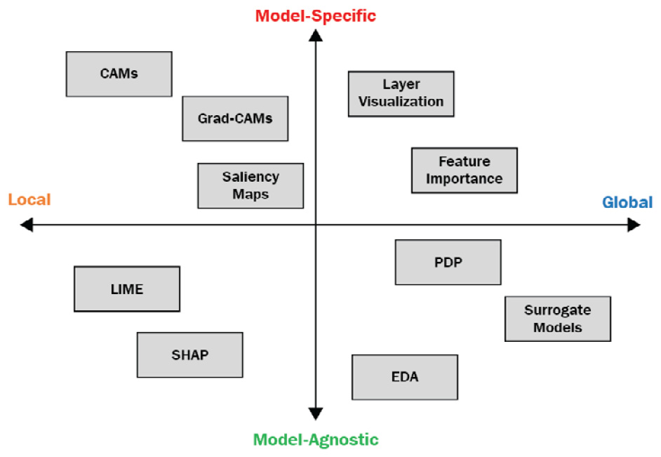
Figure 2.17 – Mapping various methods based on their explainability type

LIME and SHAP are important local and model-agnostic algorithms that are not covered in this chapter, but they will be covered in more detail later. The model explainability methods discussed in this chapter are widely used with a variety of datasets to provide different dimensions of explainability.

Summary

In this chapter, you learned about the various model explainability methods used to explain black-box models. Some of these are model-agnostic, while some are model specific. Some of these methods provide global interpretability, while some of them provide local interpretability. For most of these methods, visualizations through plots, graphs, and transformation maps are used to qualitatively inspect the data or the model outcomes; while for some of the methods, certain examples are used to provide explanations. Statistics and numerical metrics can also play an important role in providing quantitative explanations.

In the next chapter, we will discuss the very important concept of data-centric XAI and gain a conceptual understanding of how data-centric approaches can be leveraged in model explainability.

References

To gain additional information about the topics in this chapter, please refer to the following resources:

• Friedman, Jerome H. "Greedy function approximation: A gradient boosting machine." Annals of statistics (2001): https://www.researchgate.net/publication/280687718_Greedy_Function_Approximation_A_Gradient_Boosting_Machine
• Identifying outliers with the 1.5xIQR rule: https://www.khanacademy.org/math/statistics-probability/summarizing-quantitative-data/box-whisker-plots/a/identifying-outliers-iqr-rule
• Nelson rules: https://www.leansixsigmadefinition.com/glossary/nelson-rules/
• Accumulated Local Effects (ALE) – Feature Effects Global Interpretability: https://www.analyticsvidhya.com/blog/2020/10/accumulated-local-effects-ale-feature-effects-global-interpretability/
• Model-Agnostic Local Explanations using Individual Conditional Expectation (ICE) Plots: https://towardsdatascience.com/how-to-explain-and-affect-individual-decisions-with-ice-curves-1-2-f39fd751546f
• Figure 2.16: Counterfactual Visual Explanations, Goyal et al. 2019: https://arxiv.org/pdf/1904.07451.pdf
• Figure 2.13: Interpretability Beyond Feature Attribution: Quantitative Testing with Concept Activation Vectors (TCAV), Kim et al. [2018]: https://arxiv.org/abs/1711.11279
• Grad-CAM class activation visualization: https://keras.io/examples/vision/grad_cam/
• Generalized way of Interpreting CNNs using Guided Gradient Class Activation Maps!!: https://medium.com/@chinesh4/generalized-way-of-interpreting-cnns-a7d1b0178709
• Figure 2.12: Grad-CAM: Visual Explanations from Deep Networks via Gradient-based Localization, Ramprasaath et. al - https://arxiv.org/abs/1610.02391