Chapter 5: Using the Kusto Query Language (KQL)

The Kusto Query Language (KQL) is a plain-text, read-only language that is used to query data stored in Azure Log Analytics workspaces. Much like SQL, it utilizes a hierarchy of entities that starts with databases, then tables, and finally columns. In this chapter, we will only concern ourselves with the table and column levels.

In this chapter, you will learn about a few of the many KQL commands that you can use to query your logs.

In this chapter, we will cover the following topics:

• How to test your KQL queries
• How to query a table
• How to limit how many rows are returned
• How to limit how many columns are returned
• How to perform a query across multiple tables
• How to graphically view the results

Running KQL queries

For the purpose of this chapter, we will be using the sample data available in the Azure Data Explorer (ADE). This is a very useful tool for trying simple KQL commands. Feel free to use it to try the various commands in this chapter. All the information used in the queries comes from the sample data provided at https://dataexplorer.azure.com/clusters/help/databases/Samples.

If prompted, use the login credentials you would use to log in to the Azure portal. When you log in for the first time, you will see the following screen. Note that your login name may show up on the right-hand side of the header:

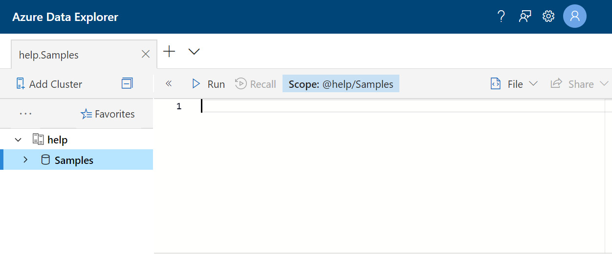
Figure 5.1 – Azure Data Explorer

In order to run the samples for this chapter, you will need to expand the Samples logs on the left-hand side of the screen and then select StormEvents. You can expand StormEvents to see a listing of fields if you want to. If you do so, your screen should look similar to the following:

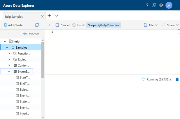
Figure 5.2 – StormEvents

To run a query, either type or paste the command into the query window at the top of the page, just to the right of the line numbered 1 in the preceding screenshot. Once the query has been entered, click on the Run button to run the query. The output will be shown in the results window at the bottom of the page.

In the following screenshot, a simple query was entered and run. The query was entered in the query window and you can see that the results are shown below it:

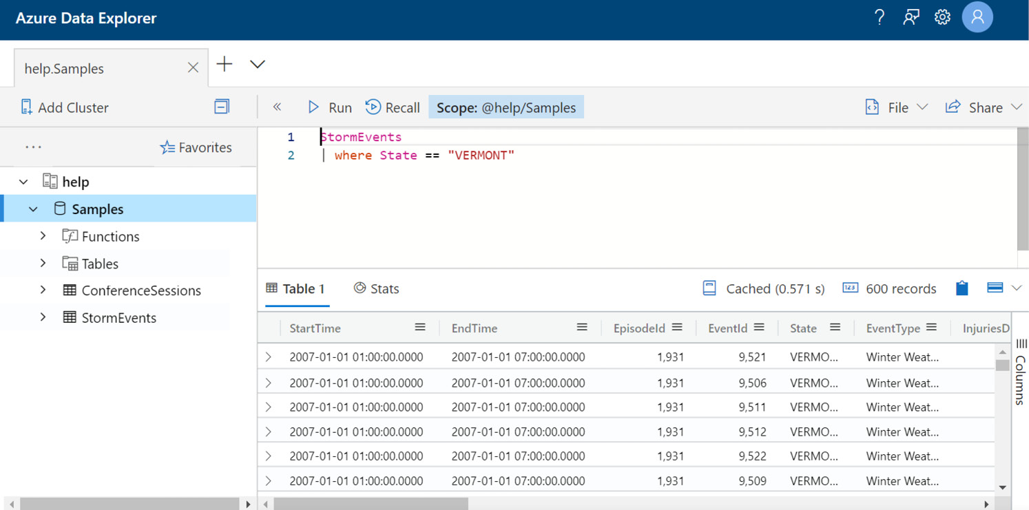
Figure 5.3 – Executed Query

There is a lot more you can do with the ADE, so feel free to play around with it. Now that you have an understanding of how we are going to run the queries and view the results, let’s take a look at some of the various commands KQL has to offer.

Introduction to KQL commands

Unlike SQL, the query starts with the data source, which can be either a table or an operator that produces a table, followed by commands that transform the data into what is needed. Each command will be separated using the pipe ( | ) delimiter.

What does this mean? If you are familiar with SQL, you would write a statement such as Select * from table to get the values. The same query in KQL would just be table, where table refers to the name of the log. It is implied that you want all the columns and rows. Later, we will discuss how to minimize what information is returned.

We will only be scratching the surface of what KQL can do here, but it will be enough to get you started writing your own queries so that you can develop queries for Azure Sentinel.

The following table provides an overview of the commands, functions, and operators we will be covering in the rest of this chapter:

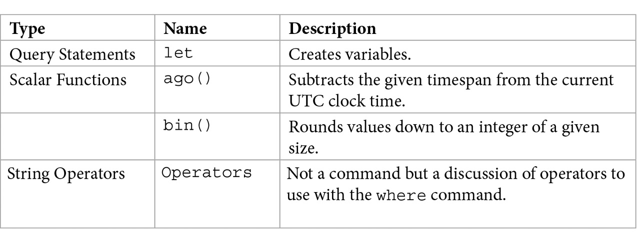
Note

For a complete list of all the KQL commands and more examples, go to https://docs.microsoft.com/en-us/azure/kusto/query/index.

Tabular operators

A tabular operator in KQL is one that can produce data in a mixture of tables and rows. Each tabular operator can pass its results from one command to another using the pipe delimiter. You will see many examples of this throughout this chapter.

The print command

The print command will print the results of a simple query. You will not be using this in your KQL queries, but it is useful for trying to figure out how commands work and what output to expect.

A simple print command such as print “test” will return a single row with the text test on it. You will see this command being used in the The bin () function section later.

The search command

As we stated earlier, to search using KQL, you just need to look at the table in the log. This will return all the columns and all the rows of the table, up to the maximum your application will return.

So, in the ADE, if you enter StormEvents into the search window and click Run, you will see a window similar to what is shown in the following screenshot. Note that there are a lot more rows available; the following screenshot just shows a small sample:

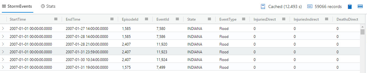
Figure 5.4 – Sampling the rows of StormEvents

If you need to search for a specific term in all the columns in all the logs in your workspace, the search command will do that for you.

If you need to find all the occurrences of York, you can use the following command:

search “York”

This will return results like what is shown in the following screenshot. Note that I have hidden some of the columns to make it easier to see that York is shown in more columns than just State:

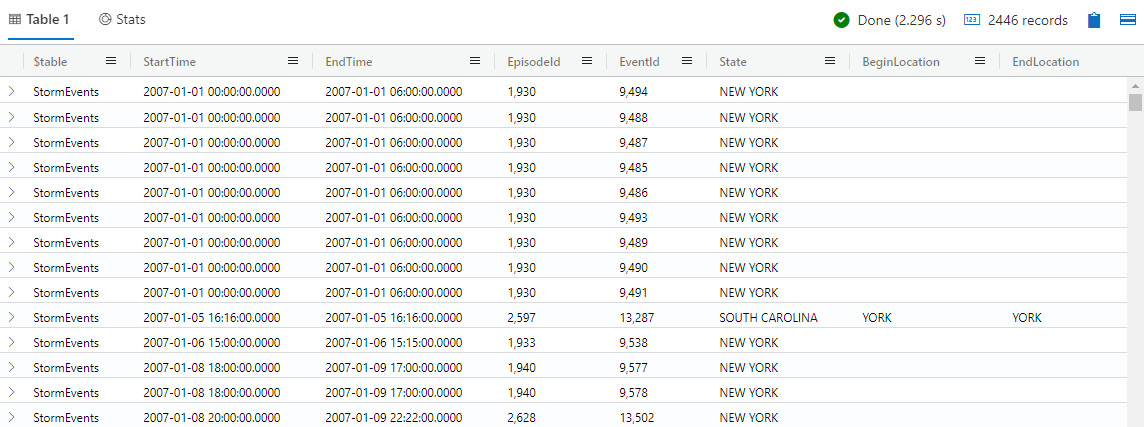
Figure 5.5 – Search command

Be warned that using the search command can take a significant amount of time to perform the query.

The where command

Recall from the screenshot from the The search command section that you get all the rows in the table when you just enter the table name, up to the maximum number of rows allowed to be returned. 99% of the time, this is not what you want to do. You will only want a subset of the rows in the table. That is when the where operator is useful. This allows you to filter the rows that are returned based on a condition.

If you want to see just those storm events that happened in North Carolina, you can enter the following:

StormEvents

| where State == “NORTH CAROLINA”

This will return all the rows where the column called State exactly equals NORTH CAROLINA. Note that == is case-sensitive, so if there was a row that had North Carolina in the State column, it would not be returned. Later, in the String operators section, we will go into more depth about case-sensitive and case-insensitive commands.

The take/limit command

There may be times when you just need a random sample of the data to be returned. This is usually so you can get an idea of what the data will look like before running a larger data query.

The take command does just that. It will return a specified number of rows; however, there is no guarantee which rows will be returned so that you can get a better sampling.

The following command will return five random rows from the StormEvents table:

StormEvents

| take 5

Note that limit is just an alias for take so that the following command is the same as the preceding command. However, it’s likely that different rows will be returned since the sampling is random:

StormEvents

| limit 5

While you may not use the limit or take commands much in your actual queries, these commands are very useful when you’re working to define your queries. You can use them to get a sense of the data that each table contains.

The count command

There may be times when you just need to know how many rows your query will return. A lot of times, this is done to get an idea of the data size you will be working with or just to see if your query returns any data without seeing the return value.

count will return the number of rows in the query. So, if we want to see the number of rows in the StormEvents table, we can enter the following:

StormEvents

| count

This will return just one column with 59,066 as the answer. Note how much faster this was than just showing all the rows in StormEvents using a basic search command and looking at the information bar to get the total. It can take around 12 seconds to process and show all the rows compared to around 0.2 seconds to get the answer when using count. The time that will be taken to perform the query may vary, but in all cases, it will be significantly faster to just get a count of the number of rows than to look at all the rows.

The summarize command

There will be times when you just need to know the total values for a specific grouping of rows. Suppose you just need to know how many StormEvents occurred for each location. The following command will show that:

StormEvents

| summarize count() by BeginLocation

This will return values like the ones shown in the following screenshot:

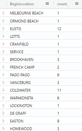
Figure 5.6 – Summarize by BeginLocation

Note that this screenshot is only showing a partial listing of the results.

You may have noticed that count, in this case, has parentheses after it. That is because count, as used here, is a function rather than an operator and, as a function, requires parentheses after the name. For a complete list of aggregate functions that can be used, go to https://docs.microsoft.com/en-us/azure/kusto/query/summarizeoperator#list-of-aggregation-functions.

The by keyword is telling the command that everything that follows are the columns that are being used in the query to perform the summary.

You can also list multiple columns if you want to have more detailed information. For instance, the following command will summarize StormEvents by State and then BeginLocation:

StormEvents

| summarize count() by State, BeginLocation

If there is more than one BeginLocation in a state, the state will be listed multiple times, as shown in the following screenshot:

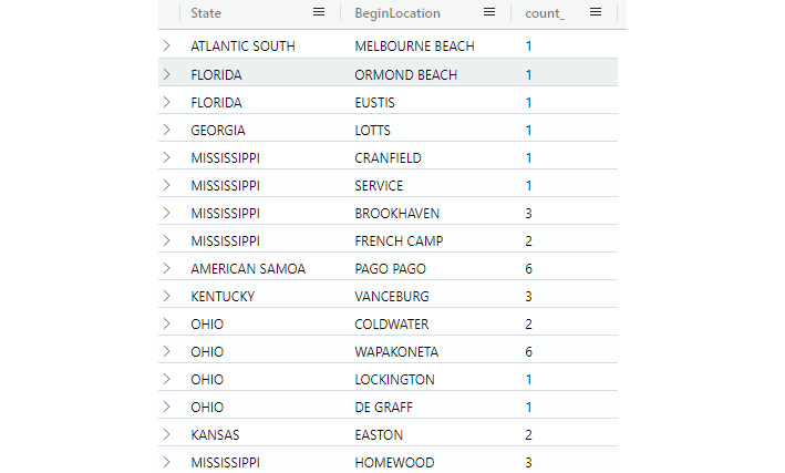
Figure 5.7 – Summarize by State and BeginLocation

Again, this screenshot is only showing a partial list of the results.

The extend command

There may be times when you need information that the table does not provide but can be generated from the data that has been provided. For example, the StormEvents table provides a start time and an end time for the event but does not provide the actual duration of the event. We know we can get the duration by subtracting the start time from the end time, but how can we tell KQL to do this?

The extend command does this. It allows you to create new columns from existing columns, or other data, such as hardcoded values. The following command will create a new column called Duration that will then be populated by the difference between the EndTime and the StartTime in each row of the StormEvents table:

StormEvents

| extend Duration = EndTime – StartTime

The following screenshot shows a sample of the output. It may not be obvious from this screenshot, but it should be noted that any column that’s created using extend will always be shown as the last column in the list, unless specifically told otherwise (more on that later):

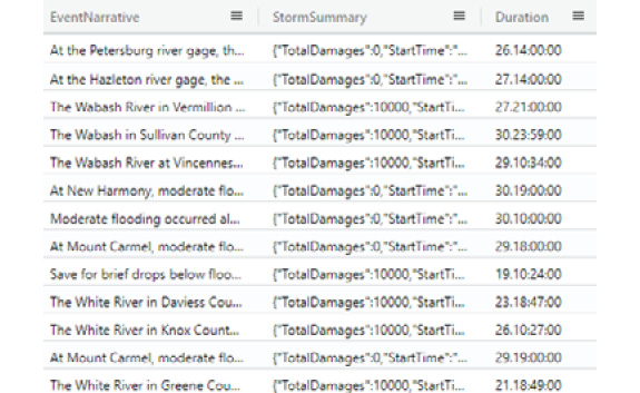
Figure 5.8 – The extend command

As we stated previously, the extend command does not need to use other columns as it can use hardcoded values as well, so the following command is perfectly valid:

StormEvents

| extend  Test = strcat(“KQL”,” rocks”)

Note that the strcat function concatenates two or more strings into one. The output will look like the following screenshot. Since we are not taking any values from the rows via a column reference, the value will always be the same, in this case, KQL rocks:

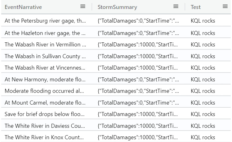
Figure 5.9 – The extend command with hardcoded values

This command will be very useful when outputting information that may exist in multiple columns but you want it to be shown in a single column.

The project command

If you don’t need to see all the columns that a query would normally show, project is used to determine what columns to show. In the following query, only StartTime, EndTime, and EventId will be shown:

StormEvents

| project StartTime, EndTime, EventId

The output is shown in the following screenshot. One item of interest is that the query took significantly less time to run than when showing all the columns:

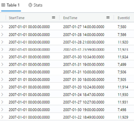
Figure 5.10 – Project command

project is like extend in that they can both create new columns. The main difference is that the extend command creates a new column at the end of the result set, while the project command creates the column wherever it is in the list of variables. It’s good practice to use the extend command for anything other than the simplest of computations to make it easier to read the query. There are two commands that produce the same results. The first command is as follows:

StormEvents

| extend Duration = EndTime - StartTime

| project StartTime, EndTime, EventId, Duration

The other command is as follows:

StormEvents

| project StartTime, EndTime, EventId, Duration = EndTime – StartTime

Here, you can see that the project command is quite useful for cleaning up the results by removing those columns you don’t care about.

The distinct command

There may be times where you get multiple instances of the same value returned but you only need to see one of them. That is where distinct comes in. It will return only the first instance of a collection of the specified column(s) and ignore all the rest.

If I run the following command, I will get a value back for all 59,066 rows and it will include many duplicates:

StormEvents

| project State

The output is shown in the following screenshot. Note the multiple occurrences of FLORIDA, MISSISSIPPI, and OHIO:

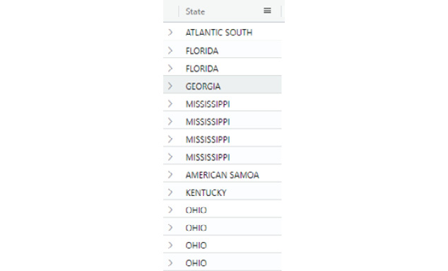
Figure 5.11 – Rows with multiple states

If we need to see just one instance of each state, we can use the following command and only get 67 rows returned to us:

StormEvents

| distinct State

This still returns the states but only one instance of each state will be returned, as shown here:

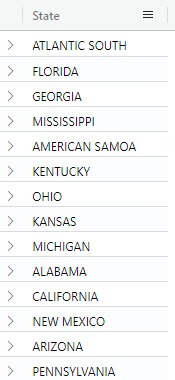
Figure 5.12 – The distinct command

By using the distinct command, you can easily see which values are in a column. This can be quite useful when building up your query. In the preceding example, you can see which states are represented in the dataset without having to scroll through all the rows if you didn’t use distinct.

The sort/order command

When you run a query, by default, the rows will be returned in whatever order they were saved into the table you are querying. If we look at the results from running the last command in the The distinct command section, the states are returned in the order the first occurrence of the state was found in the table.

Building on the command we used in the previous section, please refer to Fig 5.12 to see the output and note that the states are returned in a random order.

Most of the time, this is not what you are looking for. You will want to see the values in a specific order, such as alphabetical or based on a time value. sort will allow you to sort the output into any order you wish.

The following command will sort the output by the State column:

StormEvents

| distinct  State

| sort by State

A sample of the output is as follows:

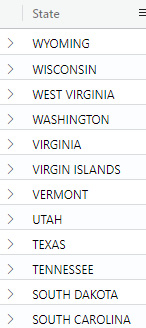
Figure 5.13 – The sort command showing states listed in descending alphabetical order

Note that the output is in alphabetical order, but it is in the default descending order. While this may be what you want, if you wanted to see the states that start with A first, you will need to specify that you want the sort to be done in ascending order. The following command shows how to do that:

StormEvents

| distinct  State

| sort by State  asc

In the following output, you can see that those states that start with A are now shown first:

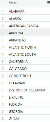
Figure 5.14 – The sort command showing states listed in ascending alphabetical order

Note that order can also be used in place of sort, so the following command will do exactly the same thing that we just saw:

StormEvents

| distinct  State

| order by State  asc

As you can see, the sort command is extremely useful when you need to see your output in a specific order, which will probably be most of the time.

The join command

The join operator will take the columns from two different tables and join them into one. In the following contrived example, all the rows from StormEvents where State equals North Carolina will be combined with the rows from FLEvents where they have a matching EventType column:

let FLEvents = StormEvents

| where State == “FLORIDA”;

FLEvents

| join (StormEvents

| where State == “NORTH CAROLINA”)

on EventType

You will use the join command quite a bit when writing your queries to get information from multiple tables or the same table using different parameters. Next, we will examine the union command and how it differs from the join command.

The union command

The union command combines two or more tables into one. While join will show all the columns of the matching rows in one row, union will have one row for each row in each of the tables. So, if table 1 has 10 rows and table 2 has 12 rows, the new table that’s created from the union will have 22 rows.

If the tables do not have the same columns, all the columns from both tables will be shown, but for the table that does not have the column, the values will be empty. This is important to remember when performing tests against the columns. If table 1 has a column called KQLRocks and table 2 does not, then, when looking at the new table that’s created by the union, there will be a value for KQLRocks for the rows in table 1, but it will be empty for the rows in table 2. See the following code:

let FLEvents = StormEvents

| where State == “FLORIDA”;

let NCEvents = StormEvents

| where State == “NORTH CAROLINA”

| project State, duration = EndTime - StartTime;

NCEvents | union FLEvents

In the following example, when looking at the rows where the state is NORTH CAROLINA, all the columns other than State and duration will be empty since the NCEvents table only has the State and duration columns. When looking at the rows where State is FLORIDA, the duration column will be empty since the FLEvents table does not have that column in it, but all the other columns will be filled out. The let command will keep the FLEvents and NCEvents variables around for later use. See the The let statement section for more information.

If we run the preceding code and scroll down a bit, we will see the output shown in the following screenshot. As you can see, most of the fields where State equals North Carolina are empty since the table that we created with the let command only contains the State and duration fields:

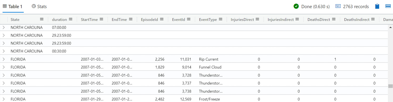
Figure 5.15 – Output of the union command

Use the union command when you need to see all the columns from the selected tables, even if some of those columns are empty in one of those tables.

The render command

The render operator is different from all the other commands and functions we have discussed in that it does not manipulate the data in any way, only how it is presented. The render command is used to show the output in a graphical, rather than tabular, format.

There are times when it is much easier to determine if something is being asked by looking at a time chart or a bar chart rather than looking at a list of strings and numbers. By using render, you can display your data in a graphical format to make it easier to view the results.

If we run the following command, we’ll get a tabular view of the data. While this is useful, it doesn’t show any outliers:

StormEvents

| project State, EndTime, DamageProperty

| where State ==”CALIFORNIA”

The partial output is as follows:

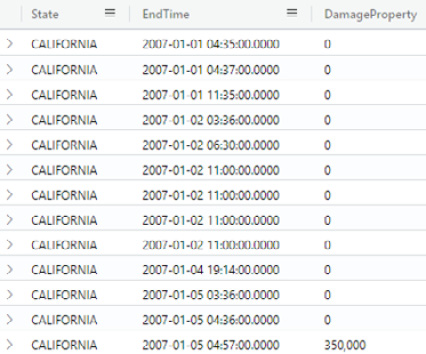
Figure 5.16 – Results shown in tabular format

While it does show there was an instance of a storm event on January 5, 2007, that caused a lot of damage, was it the one that caused the most damage? We could look through the rows and look at the DamageProperty column for each row to find this out, but there is an easier way to do this.

If we run the following command, a line chart will be generated that shows the same data but in a graphical view:

StormEvents

| project State, EndTime, DamageProperty

| where State ==”CALIFORNIA”

| render linechart

The output from this command is shown in the following screenshot. It is instantly recognizable that, while the storm we saw in January caused a lot of damage, it is nowhere near the damage caused by the storm on June 30:

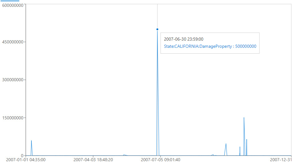
Figure 5.17 – Viewing storm damage as a graph

As shown in the preceding graph, there are times when a graphical representation of the data is more valuable than just looking at the textual output.

Information Box

The x axis is a bit misleading here with the labeling but, as you can see, when you hover your mouse over the data, the storm did occur on June 30.

Some of the other charts that can be rendered include a pie chart, an area chart, and a time chart, and each may require a different number of columns in order to present the data.

Query statement

Query statements in KQL produce tables that can be used in other parts of the query and must end with a semicolon (;). These commands, of which we will only discuss the let command here, will return entire tables that are all returned by the query. Keep in mind that a table can consist of a single row and a single column, in which case it acts as a constant in other languages.

The let statement

The let statement allows you to create a new variable that can be used in later computations. It is different than extend or project in that it can create more than just a column – it can create another table if desired.

So, if I want to create a table that contains all the StormEvents for only NORTH CAROLINA, I can use the following commands. Note the ; at the end of the let statement since it is indeed a separate statement:

let NCEvents = StormEvents

| where State == “NORTH CAROLINA”;

NCEvents

The let statement can also be used to define constants. The following command will work exactly like the one earlier. Note that the second let actually references the first let variable:

let filterstate = “NORTH CAROLINA”;

let NCEvents = StormEvents

| where State == filterstate;

NCEvents

The let statement is very powerful and one that you will use quite a bit when writing your queries.

Scalar functions

Scalar functions take a value and perform some sort of manipulation on it to return a different value. These are useful for performing conversions between data types, looking at only part of the variable, and performing mathematical computations.

The ago() function

ago is a function that is used to subtract a specific time space from the current UTC time. Remember that all times stored in the Log Analytics log is based on UTC time, unless it is a time in a custom log that is specifically designed not to be. Generally, it is safer to assume that the times stored are based on UTC time.

If I wanted to look for events in the StormEvents that ended less than an hour ago, I would use the following command. Note that this command doesn’t return any values as the times stored are from 2007:

StormEvents

| where EndTime > ago(1h)

In addition to using h for hours, you can also use d for days, among others.

The bin() function

The bin function will take a value, round down as needed, and place it into a virtual bin of a specified size. So, the print bin(7.4,1) command will return 7. It takes 7.4 and rounds down to 7. Then, it looks at the bin size, which is 1 in this case, and returns the multiple of the size that fits, which is 7. If the command is changed to print bin(7.4,4), the answer is 4. 7.4 rounded down is 7, and that fits into the second bin, which is 4. Another way of looking at this is that the first bin for this command contains the numbers 0,1,2,3, which will return a 0, the second bin is 4,5,6,7, which returns a 4 (which is why print bin(7.4,4) returns a 4), the third bin contains 8,9,10,11, which returns an 8, and so on.

This command is typically used with summarize by to group values into more manageable sizes, for example, taking all the times an activity occurred during the day and grouping them into the 24 hours in a day.

For example, if you wanted to see how many storms started during each day, you could use the following code:

StormEvents

| summarize count() by bin(StartTime,1d)

The output would appear as follows:

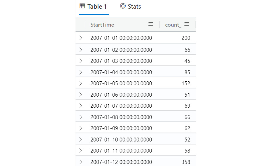
Figure 5.18 – Sample bin output

There are many more entries other than what is shown here. As you can see, bin can be quite useful to group results by date and time.

String operators

String and numeric operators are used in the comparisons of a where clause. We have already seen ==, which is a string equals operator. As we stated earlier, this is a case-sensitive operator, meaning that ABC == ABC is true but ABC == abc is false.

Note

You may need to carry out a case-insensitive comparison using =~. In this case, ABC =~ abc returns true. While there are commands to change text to uppercase or lowercase, it is good practice to not do that just for a comparison but rather do a case-insensitive comparison.

Some other string operators that can be used are as follows:

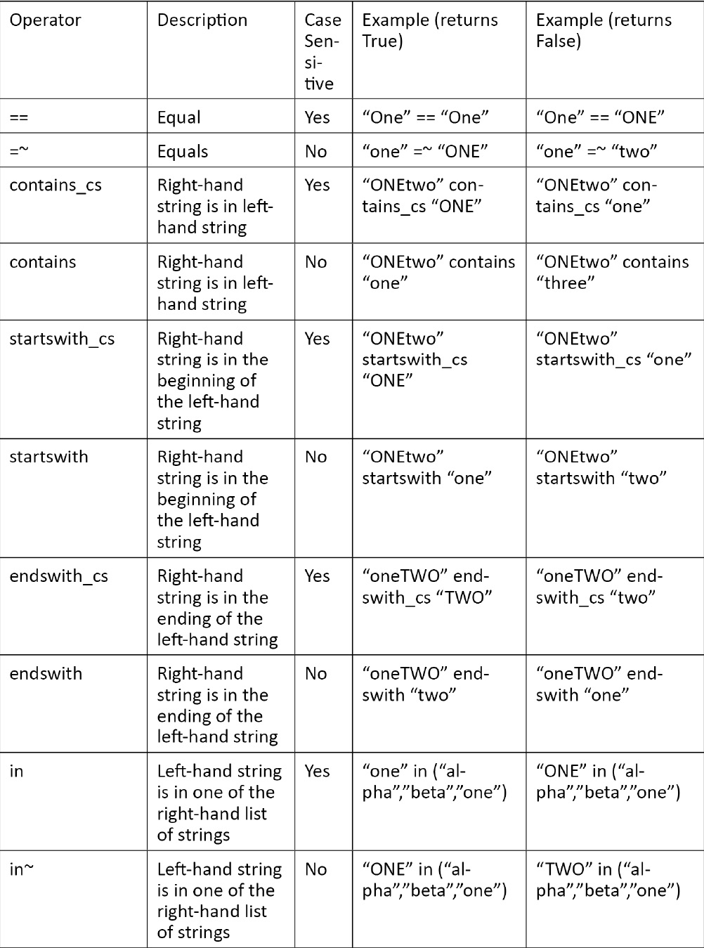
In addition, by placing ! in front of any command, that command is negated. For example, !contains means does not contain and !in means not in.

For a complete list of operators, go to https://docs.microsoft.com/en-us/azure/kusto/query/datatypes-string-operators.

Summary

In this chapter, you were introduced to the Kusto Query Language, which you will use to query the tables in your logs. You learned about some of the tabular operators, query statements, scalar functions, and string operators. Finally, we will provide some quick questions to help you understand how to use these commands to perform your queries.

In the next chapter, you will learn how to take what you learned here and use it to query logs that are stored in Azure Sentinel using the Logs page.

Questions

1. How many storms occurred in California?
2. Provide a list that shows only one occurrence of each different state.
3. Provide a list of storms that caused at least $10,000 but less than $15,000 worth of damage.
4. Provide a list of storms that show the state, amount of property damage, amount of crop damage, and the total of the property and crop damage only.

Further reading

For more information on KQL, see the following links:

• Performing queries across resources: https://docs.microsoft.com/en-us/azure/azure-monitor/log-query/cross-workspace-query#performing-a-query-across-multiple-resources
• Complete KQL command documentation: https://docs.microsoft.com/en-us/azure/kusto/query/index
• Running your KQL queries with sample data: https://portal.azure.com/#blade/Microsoft_Azure_Monitoring_Logs/DemoLogsBlade
• Additional graphical formats for queries: https://docs.microsoft.com/en-us/azure/azure-monitor/log-query/charts
• Date/time formats in KQL: https://docs.microsoft.com/en-us/azure/azure-monitor/log-query/datetime-operations#date-time-basics