
Chapter 1: Key Concepts, Notation, Set Theory, Relations, and Functions
This chapter is a general introduction to the main ideas of discrete mathematics. Alongside this, we will go through key terms and concepts in the field. After that, we will cover set theory, the essential notation and notions for referring to collections of mathematical objects and combining or selecting them. We will also think about mapping mathematical objects to one another with functions and relations and visualizing them with graphs.
In this chapter, we will cover the following topics:
- What is discrete mathematics?
- Elementary set theory
- Functions and relations
By the end of the chapter, you should be able to speak in the language of discrete mathematics and understand notation common to the entire field.
Important Note
Please navigate to the graphic bundle link to refer to the color images for this chapter.
What is discrete mathematics?
Discrete mathematics is the study of countable, distinct, or separate mathematical structures. A good example is a pixel. From phones to computer monitors to televisions, modern screens are made up of millions of tiny dots called pixels lined up in grids. Each pixel lights up with a specified color on command from a device, but only a finite number of colors can be displayed in each pixel.
The millions of colored dots taken together form intricate patterns and give our eyes the impression of shapes with smooth curves, as in the boundary of the following circle:

Figure 1.1 – The boundary of a circle
But if you zoom in and look closely enough, the true "curves" are revealed to be jagged boundaries between differently colored regions of pixels, possibly with some intermediate colors, as shown in the following diagram:

Figure 1.2 – A zoomed-in view of the circle
Some other examples of objects studied in discrete mathematics are logical statements, integers, bits and bytes, graphs, trees, and networks. Like pixels, these too can form intricate patterns that we will try to discover and exploit for various purposes related to computer and data science throughout the course of the book.
In contrast, many areas of mathematics that may be more familiar, such as elementary algebra or calculus, focus on continuums. These are mathematical objects that take values over continuous ranges, such as the set of numbers x between 0 and 1, or mathematical functions plotted as smooth curves. These objects come with their own class of mathematical methods, but are mostly distinct from the methods for discrete problems on which we will focus.
In recent decades, discrete mathematics has been a topic of extensive research due to the advent of computers with high computational capabilities that operate in "discrete" steps and store data in "discrete" bits. This makes it important for us to understand the principles of discrete mathematics as they are useful in understanding the underlying ideas of software development, computer algorithms, programming languages, and cryptography. These computer implementations play a crucial role in applying principles of discrete mathematics to real-world problems.
Some real-world applications of discrete mathematics are as follows:
- Cryptography: The art and science of converting data or information into an encoded form that can ideally only be decoded by an authorized entity. This field makes heavy use of number theory, the study of the counting numbers, and algorithms on base-n number systems. We will learn more about these topics in Chapter 2, Formal Logic and Constructing Mathematical Proofs.
- Logistics: This field makes use of graph theory to simplify complex logistical problems by converting them to graphs. These graphs can further be used to find the best routes for shipping goods and services, and so on. For example, airlines use graph theory to map their global airplane routing and scheduling. We investigate some of these issues in the chapters of Part II, Implementing Discrete Mathematics in Data and Computer Science.
- Machine Learning: This is the area that seeks to automate statistical and analytical methods so systems can find useful patterns in data, learn, and make decisions with minimal human intervention. This is frequently applied to predictive modeling and web searches, as we will see in Chapter 5, Elements of Discrete Probability, and most of the chapters in Part III, Real-World Applications of Discrete Mathematics.
- Analysis of Algorithms: Any set of instructions to accomplish a task is an algorithm. An effective algorithm must solve the problem, terminate in a useful amount of time, and not take up too much memory. To ensure the second condition, it is often necessary to count the number of operations an algorithm must complete in order to terminate, which can be complex, but can be done through methods of combinatorics. The third condition requires a similar counting of memory usage. We will encounter some of these ideas in Chapter 4, Combinatorics Using SciPy, Chapter 6, Computational Algorithms in Linear Algebra, and Chapter 7, Computational Requirements for Algorithms.
- Relational Databases: They help to connect the different traits between data fields. For example, in a database containing information about accidents in a city, the "relational feature" allows the user to link the location of the accident to the road condition, lighting condition, and other necessary information. A relational database makes use of the concept of set theory in order to group together relevant information. We see some of these ideas in Chapter 8, Storage and Feature Extraction of Trees, Graphs, and Networks.
Now that we have a rough idea of what discrete mathematics is and some of its applications, we will discuss set theory, which forms the basis for this field in the next section.
Elementary set theory
In mathematics, set theory is the study of collections of objects, which is prerequisite knowledge for studying discrete mathematics.
Definition–Sets and set notation
A set is a collection of objects. If a set A is made up of objects a1, a2, …, we write it as A = {a1, a2, …}.
Definition: Elements of sets
Each object in a set A is called an element of A, and we write an ![]() A.
A.
Definition: The empty set
Sets may contain many sorts of objects—numbers, points, vectors, functions, or even other sets.
Example: Some examples of sets
Examples of sets include the following:
- The set of prime numbers less than 10 is A = {2, 3, 5, 7}.
- The set of the three largest cities in the world is {Tokyo, Delhi, Shanghai}.
- The natural numbers are a set N = {1, 2, 3, …}.
- The integers are a set Z = {…, -3, -2, -1, 0, 1, 2, 3, …}.
- If B, C, and D are sets, A = {B, C, D} is a set of sets.
- The real numbers are written R = (-∞, ∞), which consists of the entire number line. Note that it is not possible to list the real numbers within braces, as we can with N or Z.
Definition: Subsets and supersets
A set A is a subset of B if all elements in A are also in B, and we write it as A ![]() B. We call B a superset of A. If A is a subset of B, but they are not the same set, we call A a proper subset of B, and write A
B. We call B a superset of A. If A is a subset of B, but they are not the same set, we call A a proper subset of B, and write A ![]() B.
B.
It is helpful to have an alternative notation in order to construct sets satisfying certain criteria, which we call set-builder notation, defined next.
Definition: Set-builder notation
A set may be written as {x ![]() A | Conditions}, which consists of the subset of A such that the given conditions are true.
A | Conditions}, which consists of the subset of A such that the given conditions are true.
Sometimes, sets will be expressed as {x | Conditions} when it is obvious what kind of mathematical object x is from the context.
Example: Using set-builder notation
Examples of sets constructed by set-builder notation include the following.
- The set of even natural numbers is {2, 4, 6, ...} = {n | n = 2k for some k
 N}. This is an infinite set where each element n is 2 * k, where k is some natural number belonging to the set {1, 2, 3…..}.
 - The closed interval of real numbers from a to b is {x R | a ≤ x ≤ b} = [a, b].
- The open interval of real numbers from a to b is {x R | a < x < b} = (a, b).
- The set R2 = {(x, y) | x, y R} consists of the entire 2D coordinate plane.
- The line with slope 2 and y-intercept 3 is the set {(x, y) R2 | y = 2x + 3}.
- The open ball of radius r and center (0, 0) is {(x, y) R2 | x2 + y2 < r}, which is the interior, but not the boundary of a circle.
- A circle of radius r and center (0, 0) is {(x, y) R2 | x2 + y2 = r}, which is the boundary of the circle.
- The set of all African nations is {x Nations | x is in Africa}.
There are some useful operations that may be done to pairs of sets, which we will see in the next definition.
Definition: Basic set operations
Let A and B be sets. Let's take a look at the basic operations:
- The union of sets A and B is the set of all elements in A or B (or both) and is denoted A
 B = {x | x A or x B}.
 - A union of sets A1, A2, … is denoted
 .
. - The intersection of sets A and B is the set of all elements in both A and B. It is denoted A
 B = {x | x A and x B}.
 - An intersection of sets A1, A2, … is denoted
 .
. - The complement of set A is all elements in the set that are not in A and is denoted AC = {x | x
 A}.
A}. - The difference between sets A and B is the set of all elements in A, but not B, denoted A - B = {x A | x B}.
It is often useful to represent these set operations with Venn diagrams, which are visual displays of sets. Here are some examples of the operations shown previously:
- The following displays A B:

Figure 1.3 – A ![]() B
B
- The following displays A B:

Figure 1.4 – A ![]() B
B
- The following displays Ac:
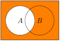
Figure 1.5 – Ac
- The following displays A – B:
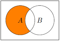
Figure 1.6 – A - B
As an example, consider the following diagram. We can use the language of set theory to describe many aspects of the diagram:
- Elements a, b, and d are in set A, which we can write as a, b, d A.
- Elements c and d are in set B, and c, d B.
- Element c is not in A, so we could write c A or c AC.
- Element d is in both A and B, or d A B.
- All four elements are in A or B (or both), so we could say a, b, c, d A B:

Figure 1.7 – Two sets with some elements
Definition: Disjoint sets
Sets A and B are disjoint (or mutually exclusive) if A ![]() B =
B = ![]() . In other words, the sets share no elements in common.
. In other words, the sets share no elements in common.
Example: Even and odd numbers
Consider sets of even natural numbers E = {2, 4, 6, ...} and odd natural numbers O = {1, 3, 5, ...}. These sets are disjoint, E ![]() O =
O = ![]() , since no number is both odd and even.
, since no number is both odd and even.
- E is a subset of the natural numbers, E
 N.
N. - O is a subset of the natural numbers, O N.
The union of E and O make up the set of all-natural numbers, E ![]() O = N.
O = N.
Theorem: De Morgan's laws
De Morgan's laws state how mathematical concepts are related through their opposites. In set theory, these laws make use of complements to address the intersection and union of sets.
De Morgan's laws can be written as follows:
- (A B)C = AC BC
- (A B)C = AC BC
The following diagrams display De Morgan's laws:

Figure 1.8 – De Morgan's laws (A ![]() B)C = AC
B)C = AC ![]() BC
BC

Figure 1.9 – De Morgan's laws (A ![]() B)C = AC
B)C = AC ![]() BC
BC
Proof:
Let's now look at the proof of this theorem:
Let x ![]() (A
(A ![]() B)C, then x
B)C, then x ![]() (A
(A ![]() B), which means x
B), which means x ![]() A and x
A and x ![]() B, or x
B, or x ![]() AC and x
AC and x ![]() BC, or x
BC, or x ![]() AC
AC ![]() BC. Thus, (A
BC. Thus, (A ![]() B)C is a subset of AC
B)C is a subset of AC ![]() BC.
BC.
Next, let x ![]() (AC
(AC ![]() BC), then x
BC), then x ![]() AC and x
AC and x ![]() BC, or x
BC, or x ![]() A and x
A and x ![]() B, then x
B, then x ![]() (A
(A ![]() B) or x
B) or x ![]() (A
(A ![]() B)C. Like the last step, we see AC
B)C. Like the last step, we see AC ![]() BC is a subset of (A
BC is a subset of (A ![]() B)C. Since (A
B)C. Since (A ![]() B)C is a subset of AC
B)C is a subset of AC ![]() BC and vice versa, (A
BC and vice versa, (A ![]() B)C = AC
B)C = AC ![]() BC.
BC.
The proof of this result is similar and is left as an exercise for the reader.
Notice that the preceding method of proof is designed to show that any element of (A ![]() B)C is an element of AC
B)C is an element of AC ![]() BC, and to show that any element of AC
BC, and to show that any element of AC ![]() BC is an element of (A
BC is an element of (A ![]() B)C, which establishes that the two sets are the same.
B)C, which establishes that the two sets are the same.
Example: De Morgan's Law
Consider two sets of natural numbers, the even numbers E = {2, 4, 6, …} and A = {1, 2, 3, 4}. If we take the set of elements in either set, or the complement of the union of the sets, we have (E ![]() A)C = {1, 2, 3, 4, 6, 8, 10, …}C = {5, 7, 9, …}.
A)C = {1, 2, 3, 4, 6, 8, 10, …}C = {5, 7, 9, …}.
De Morgan's law states that the intersection of the complements of the sets should be equal to this. Let's verify that this is true. The complements of the sets are EC = {1, 3, 5, …} and AC = {5, 6, 7, …}. The intersection of these complements is EC ![]() AC = {5, 7, 9, …}.
AC = {5, 7, 9, …}.
Definition: Cardinality
The cardinality, or size, of a set A is the number of elements in the set and is denoted |A|.
Example: Cardinality
The cardinalities of some sets are computed here:
- If A = {0, 1}, then of course its cardinality is |A| = 2, since there are two elements in the set.
- The cardinality of the set B = {x N | x < 10} is less obvious, but we can write B more explicitly. It is the set of natural numbers less than 10, so B = {1, 2, 3, 4, 5, 6, 7, 8, 9} and, clearly, |B| = 9.
- For the set of odd natural numbers, O = {1, 3, 5, ...}, we have an infinite cardinality, |O| = ∞, as this sequence goes on forever.
With our knowledge of set theory, we can now move on to learn about relations between different sets and functions, which help us to map each element from a set to exactly one element in another set.
Functions and relations
We are related to different people in different ways; for example, the relationship between a father and his son, the relationship between a teacher and their students, and the relationship between co-workers, to name just a few. Similarly, relationships exist between different elements in mathematics.
Definition: Relations, domains, and ranges
- A relation r between sets X and Y is a set of ordered pairs (x, y) where x X and y Y.
- The set {x X | (x, y) r for some y Y} is the domain of r.
- The set {y Y | (x, y) r for some x X} is the range of r.
More informally, a relation pairs element of X with one or more elements of Y.
Definition: Functions
- A function f from X to Y, denoted f : X→Y, is a relation that maps each element of X to exactly one element of Y.
- X is the domain of f.
- Elements of the function (x, y) are sometimes written (x, f(x)).
As the definitions reveal, functions are relations, but must satisfy a number of additional assumptions, in other words, every element of X is mapped to exactly 1 element of Y.
Examples: Relations versus functions
Let's look at X = {1, 2, 3, 4, 5} and Y = {2, 4, 6, …}. Consider two relations between X and Y:
- r = {(3, 2), (3, 6), (5, 6)}
- s = {(1, 4), (2, 4), (3, 8), (4, 6), (5, 2)}
The domain of r is {3,5} and the range of r is {2, 6} while the domain of s is all of X and the range of s is {2, 4, 6, 8}.
Relation r is not a function because it maps 3 to both 2 and 6. However, s is a function with domain X since it maps each element of X to exactly one element of Y.
Example: Functions in elementary algebra
Elementary algebra courses tend to focus on specific sorts of functions where the domain and range are intervals of the real number line. Domain values are usually denoted by x and values in the range are denoted by y because the set of ordered pairs (x, y) that satisfy the equation y = f(x) plotted on the Cartesian xy-plane form the graph of the function, as can be seen in the following diagram:
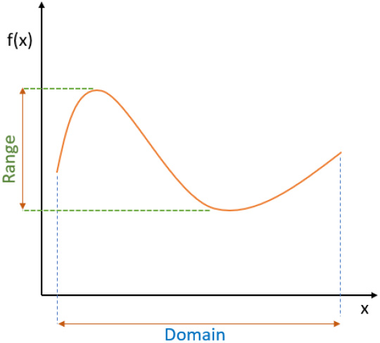
Figure 1.10 – Cartesian xy-plane
While this typical type of functions may be familiar to most readers, the concept of a function is more general than this. First, the input or the output is required to be a number. The domain of a function could consist of any set, so the members of the set may be points in space, graphs, matrices, arrays or strings, or any other types of elements.
In Python and most other programming languages, there are blocks of code known as "functions," which programmers give names and will run when you call them. These Python functions may or may not take inputs (referred to as "parameters") and return outputs, and each set of input parameters may or may not always return the same output. As such, it is important to note Python functions are not necessarily functions in the mathematical sense, although some of them are.
This is an example of conflicting vocabulary in the fields of mathematics and computer science. The next example will discuss some Python functions that are, and some that are not, functions in the mathematical sense.
Example: Python functions versus mathematical functions
Consider the sort() Python function, which is used for sorting lists. See this function applied to two lists – one list of numbers and one list of names:
numbers = [3, 1, 4, 12, 8, 5, 2, 9]
names = ['Wyatt', 'Brandon', 'Kumar', 'Eugene', 'Elise']
# Apply the sort() function to the lists
numbers.sort()
names.sort()
# Display the output
print(numbers)
print(names)
The output is as follows:
[1, 2, 3, 4, 5, 8, 9, 12]
['Brandon', 'Elise', 'Eugene', 'Kumar', 'Wyatt']
In each case, the sort() function sorts the list in ascending order by default (with respect to numerical order or alphabetical order).
Furthermore, we can say that sort() applies to any lists and is a function in the mathematical sense. Indeed, it meets all the criteria:
- The domain is all lists that can be sorted.
- The range is the set of all such lists that have been sorted.
- sort() always maps each list that can be inputted to a unique sorted list in the range.
Consider now the Python function random, shuffle(), which takes a list as an input and puts it into a random order. (Just like the shuffle option on your favorite music app!) Refer to the following code:
import random
# Set a random seed so the code is reproducible
random.seed(1)
# Run the random.shuffle() function 5 times and display the
# outputs
for i in range(0,5):
numbers = [3, 1, 4, 12, 8, 5, 2, 9]
random.shuffle(numbers)
print(numbers)
The output is as follows:
[8, 4, 9, 2, 1, 3, 5, 12]
[5, 1, 3, 8, 2, 12, 9, 4]
[2, 1, 12, 9, 5, 4, 8, 3]
[1, 2, 3, 12, 5, 8, 4, 9]
[5, 8, 9, 12, 4, 3, 2, 1]
This code runs a loop where each iteration sets the list numbers to [3, 1, 4, 12, 8, 5, 2, 9], applies the shuffle function to it, and prints the output.
In each iteration, the Python function shuffle() takes the same input, but the output is different each time. Therefore, the Python function shuffle() is not a mathematical function. It is, however, a relation that can pair each list with any ordering of itself.
Summary
In this chapter, we have discussed the meaning of discrete mathematics and discrete objects. Furthermore, we provided an overview of some of the many applications of discrete mathematics in the real world, especially in the computer and data sciences, which we will discuss in depth in later chapters.
In addition, we have established some common language and notation of importance for discrete mathematics in the form of set notation, which will allow us to refer to mathematical objects with ease, count the size of sets, represent them as Venn diagrams, and much more. Beyond this, we learned about a number of operations that allow us to manipulate sets by combining them, intersecting them, and finding complements. These give rise to some of the foundational results in set theory in De Morgan's laws, which we will make use of in later chapters.
Lastly, we took a look at the ideas of functions and relations, which map mathematical objects such as numbers to one another. While certain types of functions may be familiar to the reader from high school or secondary school, these familiar functions are typically defined on continuous domains. Since we focus on discrete, rather than continuous, sets in discrete mathematics, we drew the distinction between the familiar idea and a new one we need in this field. Similarly, we showed the difference between functions in mathematics and functions in Python and saw that some Python "functions" are mathematical functions, but others are not.
In the remaining four chapters of Part I: Core Concepts of Discrete Mathematics, we will fill our discrete mathematics toolbox with more tools, including logic in Chapter 2, Formal Logic and Constructing Mathematical Proofs, numerical systems, such as binary and decimal, in Chapter 3, Computing with Base n Numbers, counting complex sorts of objects, including permutations and combinations, in Chapter 4, Combinatorics Using SciPy, and dealing with uncertainty and randomness in Chapter 5, Elements of Discrete Probability. With this array of tools, we will be able to consider more and more real-world applications of discrete mathematics.