
Metaverse and XR systems use a lot of artificial intelligence (AI) technology in every aspect of the systems and services. For example, AI, machine learning (ML), and deep learning (DL) are used for computer vision, feature extraction and tracking, avatar and robotic control, user eye and motion tracking, speech recognition, natural language processing, sensor signal tracking, computational creativity, and future predictions (www.coursera.org/learn/deep-learning-business).
Multimedia systems also use AI technology everywhere, which include user recommendation systems, enterprise resource planning (ERP) and management, server streaming speed control, video and audio adaptive quality control, illegal image or information automatic detection, automated privacy protection, as well as automated network and cloud security monitoring and cyberattack defense control.
DL enables extreme levels of precision and reliable automated control and is self-learning and adaptable to changes, which is why metaverse XR and multimedia services use DL abundantly.
Backpropagation Supervised Learning
Deep Learning with Recurrent Neural Network (RNN)
Deep Learning with Convolutional Neural Network (CNN)
Performance of AI Systems
Performance of CNN at the ImageNet Challenge
Performance of RNN in Amazon’s Echo and Alexa
Advanced RNN and CNN Models and Datasets

A concentric illustration of artificial intelligence at the outer, machine learning in the middle, and deep learning at the inner.
Relation Between AI, ML, and DL
AI is intelligence performed by a computing system. AI systems are designed to mimic natural intelligence, which is intelligence performed by a living being, such as a human or animal (https://en.wikipedia.org/wiki/Artificial_intelligence). Modern AI systems are able to exceed the performance of human intelligence in specific tasks, as explained with examples in later sections of this chapter. AI technology enables a computing system to make an intelligent decision or action and enables an intelligent agent (e.g., hardware, software, robot, application) to cognitively perceive its environment and correspondingly attempt to maximize its probability of success of a target action. AI has been used in making optimal decisions (or faster suboptimal decisions) for many types of control systems. Various forms of AI technology can be found in optimization theory, game theory, fuzzy logic, simulated annealing, Monte Carlo experiments and simulation, complex theory, etc.
ML is an AI technique that can enable a computer to learn without being explicitly programmed. ML has evolved from pattern recognition and computational learning theory in AI. ML provides the functionality to learn and make predictions from data.
DL is a ML technique that uses multiple internal layers (hidden layers) of nonlinear processing units (artificial neurons) to conduct supervised or unsupervised learning from data. DL is commonly implemented using an artificial neural network (NN).

The diagram of a neuron with dendrites, a nucleus, soma, myelin sheaths, and axon and axon terminals. The messages flow from dendrites to axon terminals.
Neuron (i.e., Nerve Cell)

An illustration of synaptic connections between the axon terminals of the neuron and the dendrites of other neurons.
Neurons Transferring Signals over Synaptic Connections
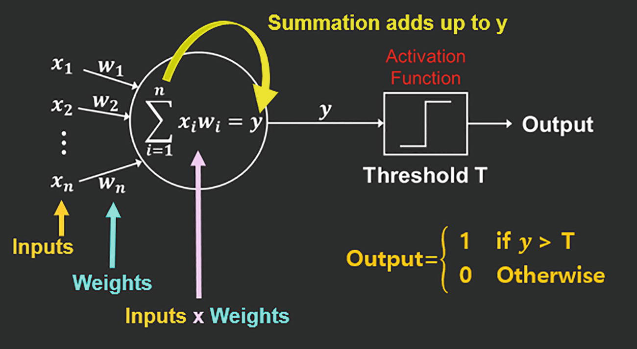
An illustration of inputs, weights, inputs into weights, and inputs into weights' summation adds up to y, threshold T, activation function, and output.
Artificial Neuron (i.e., Nerve Cell) Used in DL and Artificial NNs

Logistic sigmoid

Softplus ζ(y) = log (1 + exp (y))
Rectified linear unit (ReLU) g(y) = max (0, y)

A graph for sigma y versus y represents a diagonally placed s-shaped line. The top and bottom of the s-shaped line are flatlined.
Logistic Sigmoid Activation Function

A graph for zeta y versus y represents a line that begins at 0 on the y-axis, moves horizontally for some distance, and ascends diagonally to reach the top right corner.
Softplus Activation Function

A graph for g y versus y represents a line that begins at 0 on the y-axis, moves horizontally for some distance, and ascends diagonally to reach the top right corner.
ReLU Activation Function
DL NNs are formed using perceptrons and multilayer perceptrons (MLPs). A perceptron is a ML algorithm that conducts supervised learning of linear (binary) classification. Perceptrons are trained to determine if an input (tensor, vector, or scalar value) belongs to one class or another. A MLP is a feed forward NN that is formed of multiple layers of perceptrons, where each layer may use multiple perceptrons in parallel. MLPs use backpropagation based supervised learning to train the outputs (to accurately conduct nonlinear classification). More details on backpropagation supervised learning are described in the following section.
Original inputs a1, a2, a3
Softmax outputs

Constraint satisfied

 =1
=1
 ) combined in the following form of
ML and DL systems also use AutoEncoders. An AutoEncoder (or AutoAssociator) is a NN used to learn the characteristics of a dataset such that the representation (encoding) dimensionality can be reduced. The simplest form of an AutoEncoder is a feedforward nonrecurrent neural network (non-RNN).
Backpropagation Supervised Learning

A diagram of a structure with weights of W subscripts 1 and 2. The right diagram depicts A, B, C, and D in the corners, along with a right slating line that passes close to A.
Neuron (Single Layer) with Two Inputs and Two Weights (i.e., w1, w2) (Left Side) and the Achievable Decision Boundaries (Right Side)

A diagram of a structure with weights of W subscripts 1, 2, 3, and 4. The right diagram depicts A, B, C, and D in the corners and two left-slanting lines enclosing A and D.
Two-Layer NN Using Three Neurons with Four Weights (i.e., w1, w2, w3, w4) (Left Side) and the Achievable Decision Boundaries (Right Side)

A diagram of a structure with weights of W subscript 1 to 8. The right diagram depicts A, B, C, and D in the corners, and A and D are enclosed by trapezoids.
Three-Layer NN Using Five Neurons with Eight Weights (i.e., w1, w2, w3, w4, w5, w6, w7, w8) (Left Side) and the Achievable Decision Boundaries (Right Side)

An illustration of the input, hidden, and output layers along with their connections in the middle region, which are regions for weight training.
Generalized NN Model and Weight Training Region

An illustration of the input layer, the hidden layers, and the output layers and their connections.
DL NN with Multiple Hidden Layers
Learning is how DL trains the weights of the hidden layers to make the NN intelligent. DL NN learning (training) methods include supervised learning, unsupervised learning, semi-supervised learning, and reinforcement learning. Supervised learning is a training method that uses labeled data. Labeled data is input data that has the desired output value included. This is like an exam problem where the answer is used with the problem to educate (train) the student (NN). Unsupervised learning is a training method that uses unlabeled data (no desired outputs are used). Semi-supervised learning is a training method that uses both labeled data and unlabeled data (www.deeplearningbook.org/). Reinforcement learning is a training method that uses feedback (reward) of the output to make optimal decisions but does not use any labeled data.
Among these learning methods, supervised learning using backpropagation training is used the most for metaverse XR and multimedia systems, so we will focus on this DL technique. Backpropagation is used to train the perceptrons and MLPs. Backpropagation uses training iterations where the error size as well as the variation direction and speed are used to determine the update value of each weight of the NN.
- 1.
Forward propagate the training pattern’s input data through the NN.
- 2.
NN generates initial output values.
- 3.
Use the output value and labeled data desired output value to compute the error value. Use the error value and input value to derive the gradient of the weights (size and +/- direction of change) of the output layer and hidden layer neurons.
- 4.
Scale down the gradient of the weights (i.e., reduce the learning rate), because the learning rate determines the learning speed and resolution.
- 5.
Update weights in the opposite direction of the +/- sign of the gradient, because the +/- sign of the gradient indicates +/- direction of the error.
- 6.
Repeat all steps until the desired input-to-output performance is satisfactory.

An illustration of the input, hidden, and output layers mentions backpropagate errors to train N N weights. The current output minus the desired output equals an error.
Supervised Learning Using Backpropagation Training
Backpropagation learning uses the gradient to control the weight values. Gradient is the derivative of a multivariable (vector) function. Gradients point in the direction of the greatest rate of increase of the multivariable function, and the magnitude of the gradient represents the slope (rate of change) in that direction. So, updating the hidden layer weight values considering the direction and magnitude of the current gradient can significantly help to minimize the error output. However, because each weight of the NN is used in the calculation of various other inputs, the size of a weight update has to be small in each training iteration. This is because a big change in one weight may mess up the weights that were properly trained to match the other input to output values.
Deep Learning with RNN
Recurrent neural network (RNN) deep learning is the most powerful AI technology for speech recognition, speech-to-text (STT) systems, as well as sensor data sequence analysis and future predicting. Therefore, almost all XR, game, metaverse, and multimedia systems use RNN technology. A few representative examples of smartphone apps that use RNN speech recognition and STT technology include Apple Siri, Amazon Alexa, Google Assistant and Voice Search, and Samsung Bixby and S Voice. In addition, RNN is used for handwriting recognition and almost any type of sequential or string data analysis. RNN is also capable of software program code generation, in which a RNN system is used to automatically generate computer programming codes that can serve a predefined functional objective (www.deeplearningbook.org/).

An illustration of X subscript 1 to 6 as inputs, S 2 S learning in the middle, and Y subscript 1 to 4 as outputs.
RNN S2S Learning System Example with Six Inputs and Four Outputs
- 1.
Data enters the input layer.
- 2.
Representation of the data in the input layer is computed and sent to the hidden layer.
- 3.
Hidden layer conducts sequence modeling and training in forward and/or backward directions.
- 4.
Multiple hidden layers using forward or backward direction sequence modeling and training can be used.
- 5.
Final hidden layer sends the processed result to the output layer.

A diagram of the input layer followed by sequence modeling, the R N N layer-hidden layer, related to memory, and the output layer.
Forward RNN System Example

A diagram of the input layer followed by sequence modeling, the R N N layer-hidden layer, related to memory, and the output layer. The hidden layer's flow is to the left.
Backward RNN System Example

An illustration of the input layer, the hidden layers composed of R N N layers, and the output layer.
S2S Deep Learning RNN Example
Because RNNs and CNNs use many hidden layers in their NNs for data analysis, they are called deep neural networks (DNNs), and because deep neural networks are used to learn the data pattern and semantics (and much more) through training, the overall technology is called deep learning (DL). The number of hidden layers required as well as the input, output, and hidden layer structures are based on the data type and target application results needed.
The RNN data analysis applies a representation process to the input data, which is similar to subsampling. As the data sequentially enters the RNN through the input layer, a small dataset (in array or matrix form) is formed, and data representation is applied to extract the important data that characterizes the dataset in the best way. This process is repeated as the data continuously enters the RNN input layer. Representation is a nonlinear down-sampling process that is effective in reducing the data size and filtering out the noise and irregular factors that the data may have. The RNN “representation” process is similar to the “subsampling” and “pooling” process used in CNN, which will be described in the following section of this chapter when describing XR image processing techniques using deep learning. Some examples of representation are presented in the following.

An illustration of a square with three columns and three rows of numbers. The number in the middle is five and is highlighted.
RNN “Center” Representation Example, Where the Center Value of the DataSet Is Selected
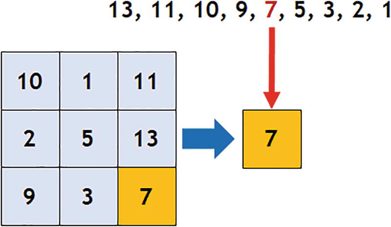
An illustration of a square with three columns and three rows of numbers. The number in the bottom right corner is 7 and is highlighted.
RNN “Median” Representation Example, Where the Median Value of the DataSet Is Selected
The median method first lines up the dataset values in order of the largest to the smallest and then selects the value in the middle. For example, in Figure 4-19, if we line up the numbers in the dataset from largest to the smallest, then we get 13, 11, 10, 9, 7, 5, 3, 2, 1 in which 7 is in the middle of the number sequence, so the median value is 7.

An illustration of a square with three columns and three rows of numbers. The number in the middle of the left column is 13 and is highlighted.
RNN “Max Pooling” Representation Example, Where the Maximum Value of the DataSet Is Selected

An illustration of a square with three columns and three rows of numbers. The average number in the square is 6.7.
RNN “Average” Representation Example, Where the Average Value of the DataSet Is Selected

A diagram of two squares. The rows and columns on the left square are filled with w subscript 1 to 9, and those on the right square with d subscript 1 to 9, their multiplications equal v.
RNN “Weighted Sum” Representation Example, Where the Resulting Weighted Sum Value Is v

A diagram of a context column with the values c subscript 1 to c subscript 4 and a data square of three rows and three columns with x subscript 1 to 9 in it.
RNN Hidden Layer Context-Based Projection Example

An illustration of three squares, each with three rows and three columns. The context, current input, and past information are also depicted.
Larger-Scale RNN Hidden Layer Context-Based Projection Example

An illustration of inputs X subscripts 1, 2, and 3, attention, and output X subscript s.
RNN Softmax Transfer with Attention Data Processing Example, Where the Attention Values A1, A2, and A3 Represent the Importance of the DataSet
In the RNN process of representation with attention, the Softmax transfer is used frequently to transfer the values a1, a2, and a3, respectively, into  ,
,  , and
, and  .
.
The attention values A1, A2, and A3 represent the importance of the input datasets X1, X2, and X3.
 ,
,  , and
, and  to transform each dataset, where an element-wise multiplication is applied to the outputs 1’, 2’, and 3’ that are shown in Figure 4-26.
An illustration of gridded squares, values, attention values, input data sets, weight values, SoftMax output values, and X subscript s.
RNN Softmax Transfer with Attention and Element-Wise Multiplication Data Processing Example

An illustration of input of x subscript t, input gate, forget gate, output gate, self-loop, state, and output of h subscript t.
RNN LSTM System Example
The RNN forget gate (which is also called the recurrent gate) helps to prevent backpropagated errors from vanishing (called the vanishing gradient problem) or exploding (called the divergence problem). In addition, it enables errors to flow backward through an unlimited number of virtual layers (VLs) extending the memory characteristics.
LSTM RNN systems are very effective on data sequences that require memory of far past events (e.g., thousands of discrete time steps ago) and perform well on data sequences with long delays and mixed signals with high and low frequency components.
LSTM RNN applications are extensive, which include XR system sensor analysis, STT, speech recognition, large-vocabulary speech recognition, pattern recognition, connected handwriting recognition, text-to-speech synthesis, recognition of context sensitive languages, machine translation, language modeling, multilingual language processing, automatic image captioning (using LSTM RNN + CNN), etc.
Deep Learning with CNN
Deep learning with convolutional neural network (CNN) is commonly used in image processing and feature detection and tracking in metaverse XR and multimedia systems. CNN systems are based on a feed forward NN and use multilayer perceptrons (MLP) for this process. CNN was designed based on animal visual cortexes, where individual vision neurons progressively focus on overlapping tile shape regions. Vision tile regions sequentially shift (convolution process) to cover the overall visual field.
Deep learning CNN techniques became well known based on an outstanding (winning) performance of image recognition at the ImageNet Challenge 2012 by Krizhevsky and Hinton from the University of Toronto, which is described in further details in a following section of this chapter (www.image-net.org/challenges/LSVRC/). CNNs need a minimal amount of preprocessing and use rectified linear units (ReLU) activation functions more often (i.e., g(y) = max (0, y)). CNNs are used in image/video recognition, recommender systems, natural language processing, Chess, Go, as well as metaverse XR devices and multimedia systems.

An illustration of input, feature maps, f maps, convolutions, subsampling, fully connected, and output.
CNN Structure

An illustration of a cube with a cuboid in its center. The cuboid has five circles along its long side face.
Example of the CNN Convolution Process
Feature maps are made from the activation maps of the filters. The number of learnable filters/kernels (and how the data, weight training, bias values, etc. are used) in the convolution process determines how many feature maps are generated after convolution.
Subsampling uses a selecting operation (pooling) on the feature maps. Subsampling is a nonlinear down-sampling process that results in smaller feature maps. The CNN subsampling process is similar to the RNN representation process. The most popular subsampling schemes (many exist) include median value, average value, and max pooling.

An illustration of a square with rows and columns filled with numbers, and the average of the numbers 6 and 4 in the top right is 5.
Subsampling Example Based on the Median Value

An illustration of a square with rows and columns filled with numbers, and the average of the numbers in the top left is 4.
Subsampling Example Based on the Average Value

An illustration of a square with rows and columns filled with numbers, and the maximum value among the numbers on the top left is 8.
Subsampling Example Based on the Maximum Value

An illustration of the flow from convolutions to L C N to pooling.
Example of the LCN and Pooling Process Following the Convolution Process
Additional techniques used in CNNs include the dropout, ensemble, bagging, and pooling processes, which are explained in the following.
The dropout process helps in training neurons to properly work even when other neurons may not exist (neuron failure). Therefore, the dropout process makes the CNN more robust to noise and erroneous data. In the dropout process, on each iteration, selected neurons are randomly turned off based on a probability model. The dropout process is applied to the output layer which is in the form of a multilayer perceptron (MLP) that is fully connected to the previous hidden layer. Outputs are computed with a matrix multiplication and biased offset.
Ensemble models are often used in CNNs to improve the accuracy and reliability by providing an improved global image of the data’s actual statistics. Ensembles are created by repeated random sampling of the training (labeled) data.
Bagging uses multiple iterations of training the CNN with training/labeled data that has random sample replacements. After training, the results of all trained models of all iterations are combined.
Performance of AI Systems
AI technology has radically evolved, such that on specific tasks an AI system can outperform humans, even the best experts. A representative example of humans competing with AI started with IBM’s Deep Blue. In 1996, Deep Blue lost in a six-game match to the chess world champion Garry Kasparov. After being upgraded, Deep Blue won its second match (i.e., three games won with one draw) with Garry Kasparov in 1997. The estimated processing capability of IBM’s Deep Blue is 11.4 GFLOPS. Afterward, the technology of AI computers evolved such that AI computers commonly beat chess Grand Masters. As a result, separate from the World Chess Federation (FIDE) Ratings (for chess Grand Masters), the Computer Chess Rating Lists (CCRL) was formed in 2006 so chess fans and AI programmers could compare the performance of various AI engines in chess competitions (https://en.wikipedia.org/wiki/Deep_Blue_(chess_computer)).
Another representative example of an open-domain Question-Answering (QA) AI system beating the best human contestants happened on the television quiz show “Jeopardy!” on January 14th of 2011, when the IBM Watson QA AI system beats two Jeopardy! top champions in a two-game competition (https://en.wikipedia.org/wiki/IBM_Watson). Jeopardy! is a television quiz show in the United States that debuted on March 30th of 1964 and is still very popular. For this competition, the IBM Watson QA system went through over 8,000 independent experiments that were iteratively processed on more than 200 8-core servers that were conducted by 25 full-time researchers/engineers for this Jeopardy! match (www.ibm.com/support/pages/what-watson-ibm-takes-jeopardy).
Watson is an open-domain QA problem solving AI system made by IBM. Watson uses the deep learning QA (DeepQA) architecture for QA processing. The QA system requirements include information retrieval (IR), natural language processing (NLP), knowledge representation and reasoning (KR&R), machine learning (ML), and human-computer interface (HCI). DeepQA is a combination of numerous analysis algorithms, which include type classification, time, geography, popularity, passage support, source reliability, and semantic relatedness.
A more recent example of humans competing against DL computers is the Google’s DeepMind AlphaGo system that beats the world top ranking Go players during 2015 to 2017. The AlphaGo Master system (used in 2017) was equipped with a second generation (2G) tensor processing unit (TPU) that has a processing capability of 11.5 PFLOPS (i.e., 11.5×10¹⁵ FLOPS). A TPU is a more advanced hybrid system form of multiple central processing units (CPUs) and graphics processing units (GPUs) combined for advanced DL processing (www.nature.com/articles/nature16961).
CPUs are used to execute computations and instructions for a computer or smartphone, which are designed to support all process types. A GPU is a custom-made (graphics) processor for high-speed and low power operations. GPUs are commonly embedded in computers and smartphone video cards, motherboards, and inside system on chips (SoCs).
When describing IBM’s Deep Blue or Watson, the term FLOPS was used, which is a unit that is used to measure a computer’s performance. FLOPS stands for “FLoating-Point Operations Per Second” which represents the number of floating-point computations that a computer can complete in a second. For modern computers of smartphones, the unit GFLOPS is commonly used, which stands for Giga FLOPS, in which a Giga=Billion=109. Another unit that is used to measure a computer’s performance is IPS which stands for “Instructions per Second” which represents the number of operations that a computer can complete in a second. For modern computers or smartphones, the unit MIPS is commonly used, which stands for Millions of IPS. Humans are extremely versatile, but are not good in FLOPS performance, only reaching an average of 0.01 FLOPS = 1/100 FLOPS of a performance. 0.01 FLOPS means that it will take an average of 100 seconds to conduct one floating-point calculation. This may be shocking to you because this is too slow, but in your head without using any writing tools or calculator, try to compute the addition of two simple floating-point numbers “1.2345 + 0.6789” which results in 1.9134. You may have been able to complete this quickly, but for an average person, it is expected to take an average of 100 seconds to complete this floating-point calculation. Other numbers that can be used to approximately characterize the human brain includes 2.5 PB (i.e., 2.5×10¹⁵ Bytes) of memory running on 20 W of power.
In terms of FLOPS comparison, approximately humans can perform at a 0.01 FLOPS level, modern smartphones and computers are in the range of 10~300 GFLOPS, and TPU 2G (which was used in the Google’s DeepMind AlphaGo Master system in 2017) can provide an approximate 11.5 PFLOPS (i.e., 11.5 × 10¹⁵ FLOPS) performance.
Performance of CNN at the ImageNet Challenge
The performance level of CNN image technology is explained in this section, where the ImageNet Large Scale Visual Recognition Challenge (ILSVRC) is the original and best example. ILSVRC was an annual contest that started in 2010 focused on object category classification and detection. ILSVRC was called the “ImageNet Challenge” for short. There were three main challenges used to benchmark large-scale object recognition capability. There was one “Object Localization (top-5)” competition and two “Object Detection challenges” where one was for image detection and the other was for video detection. The “Object Localization (top-5)” was the original competition of ILSVRC. The other two Object Detection challenges were included into ILSVRC later.
The ILSVRC used a training dataset size of 1.2 million images and 1,000 categories of labeled objects. The test image set consisted of 150,000 photographs. For the Object Localization (top-5) contest, each competing AI program lists its top 5 confident labels based on each test image in decreasing order of confidence and bounding boxes for each class label. Each competing program was evaluated based on accuracy of the program’s localization labeling results, the test image’s ground truth labels, and object in the bounding boxes. The program with the minimum average error was selected as the winner (https://en.wikipedia.org/wiki/ImageNet).
As the amount of training will influence the level of learning, there were very strict participant’s program requirements. Based on the program requirements, each team (participating AI program) is allowed two submissions per week, where there is no regulation on the number of neural network layers that can be used in a contestant’s AI program. The learning scheme and parameters had to be based only on the training set.

A bar graph of the highest value of 28.2 is for I L S V R C 2010 N E C America. The deep learning C N N points at I L S V R C 2012 AlexNet.
ILSVRC ImageNet “Object Localization (Top-5)” Competition Annual Winners and Accuracy Performance. The Numbers in the Graph Are the Average Error Percentage Values. The Average 5.1% Human Error Performance Was Included in the Figure as a Reference. During ILSVRC 2015, Microsoft’s ResNet Exceeded the Human Average Performance for the First Time
The 2014 winner was Google’s GoogleNet (Inception-v1) which achieved a 93.3% accuracy in the Object Localization (top-5) competition. This was the first time a computer was able to exceed the 90% accuracy level. GoogleNet used a 22-layer DL neural network with 5 million parameters and trained for 1 week on the Google DistBelief cluster.
The 2015 winner was Microsoft’s ResNet, which achieved a 96.5% accuracy in the Object Localization (top-5) competition. This is the first time a computer program was able to exceed the 94.9% human accuracy level. ResNet used a 152-layer DL neural network that was trained for approximately 3 weeks on 4 NVIDIA Tesla K80 GPUs using a combined processing capability of 11.3 BFLOPs. By 2017, among the 38 competing teams, 29 teams achieved an accuracy exceeding 95%.
Performance of RNN in Amazon’s Echo and Alexa
In order to demonstrate how deep learning RNN can be used, the operations of the Echo and Alexa are described in the following. Amazon Echo is a voice controlled intelligent personal virtual assistant, where Alexa is accessible through the Echo smart speaker. Alexa is a cloud-based AI personal assistant developed by Amazon that requires network connection to the Amazon cloud, which is a cloud offloading system. Alexa is used in the Echo and Echo Dot products. More recent Echo product information can be found at www.amazon.com/smart-home-devices/b?ie=UTF8&node=9818047011.
In November of 2014, the Amazon Echo was released along with Alexa services at a price of $199 for invitation and $99 for Amazon Prime members. A smaller version of the Amazon Echo device is the Echo Dot device, where the first-generation device was released in March of 2016 and the second-generation device was released in October of 2016. The Echo system uses a seven-microphone array built on the top of the device, and acoustic beamforming and noise cancellation is applied for improved voice recognition capability. The seven-microphone array enables high-quality natural language processing (NLP), which is used to match the user’s voice or text as input, so the Alexa system could provide automated services requested by the user. The Alexa virtual assistant is always-on and always-listening to support the voice activated questions and answering (QA) system.

An illustration of the flow from the user to the Echo, Alexa service platform, and skill code.
Alexa Operations Initiated by the User’s Voice Through the Echo Device
Alexa’s Skills include a library of AI based functions that can assist in finding product information (type, volume, profit), marketing progress, and results search. The Alexa Skills Kit (ASK) is a developer kit used to create new custom Skills for Echo and Echo Dot.
The DL speech recognition system is triggered when the user speaks into the Echo system. The Echo’s voice recognition system detects trigger words and required Skills.
The Echo sends the user’s request to the Alexa Service Platform (ASP). The ASP uses its DL RNN speech recognition engine to detect words of intent and parameters.
The ASP sends a JavaScript Object Notation (JSON) text document (including the intent and parameters) to the corresponding Skill on the Alexa Cloud using a Hypertext Transfer Protocol (HTTP) request.

An illustration of the flow from skill code to the Alexa service platform, smartphone, echo, and user.
Skill Code Working with the ASP and Echo to Complete the user’s Request, and Smartphone Notices (Popup Cards) Can Be Received as an Option
Next, Alexa makes a Response JSON document and sends it to the ASP. This Response JSON document includes the text of Alexa’s reply to the user. As an option, the smartphone app Popup Card info can be used, in which the Popup Card includes the markup text and image URL. The ASP voice replies to the user. Optional settings can make the smartphone app popup card show up on the user’s smartphone.
Advanced RNN and CNN Models and Datasets
More advanced RNN and CNN models as well as benchmarkable deep learning datasets exist. However, due to space limitations of this chapter, a list of the advanced algorithms and datasets as well as their website links is provided to enable the reader to study more.
MSCOCO (https://cocodataset.org/#home)
PASCAL VOC (http://host.robots.ox.ac.uk/pascal/VOC/)
CIFAR-10, CIFAR-100 (www.cs.toronto.edu/~kriz/cifar.html)
ImageNet (https://image-net.org/index.php)
End-to-end speech recognition with RNN (https://proceedings.mlr.press/v32/graves14.html).
Deep speech 2 (http://proceedings.mlr.press/v48/amodei16.pdf).
Listen, attend, and spell (https://arxiv.org/abs/1508.01211).
Sequence transduction with RNN (https://arxiv.org/abs/1211.3711).
Streaming end-to-end speech recognition (https://storage.googleapis.com/pub-tools-public-publication-data/pdf/9dde68cba3289370709cee41e9bd4e966e4113f2.pdf).
Neural transducer (https://arxiv.org/pdf/1511.04868.pdf).
Monotonic Chunkwise Attention (https://arxiv.org/abs/1712.05382).
- You Only Look Once (YOLO) algorithms
- Region with CNN (R-CNN) algorithms
Fast R-CNN (https://dl.acm.org/doi/10.1109/ICCV.2015.169)
Faster R-CNN (https://ieeexplore.ieee.org/document/7485869)
Cascade R-CNN (https://ieeexplore.ieee.org/document/8578742)
Single Shot MultiBox Detector (SSD) (https://arxiv.org/pdf/1512.02325.pdf)
RefineDet (https://arxiv.org/abs/1711.06897)
RetinaNet (https://ieeexplore.ieee.org/document/8237586)
Software architecture- and processing method-wise, image recognition deep learning algorithms can be divided into one-stage methods and two-stage methods. One-stage methods include SSD, RetinaNet, YOLOv1, YOLOv2, YOLOv3, YOLOv4, and Scaled-YOLOv4 (www.jeremyjordan.me/object-detection-one-stage). Two-stage methods include FPN, R-CNN, Fast R-CNN, Faster R-CNN, Mask R-CNN, Cascade R-CNN, and Libra R-CNN (https://medium.com/codex/a-guide-to-two-stage-object-detection-r-cnn-fpn-mask-r-cnn-and-more-54c2e168438c).
Summary
This chapter introduces AI and deep learning technologies, including the internal functions of RNN and CNN systems. The history of AI and deep learning system achievements is described, including the more recent ImageNet Challenge (for CNN technology) and Amazon’s Echo and Alexa (for RNN technology). The chapter also includes a list of advanced RNN and CNN models and datasets. AI and deep learning technologies will continue to be extensively used in metaverse services, XR devices, and multimedia streaming systems, which include sensor/image signal analysis, video/audio adaptive quality control, recommendation systems, enterprise resource planning (ERP), automated management, server control, security, as well as privacy protection. In the following Chapter 5, details of video technologies used in metaverse XR and multimedia systems are introduced, which include the H.264 Advanced Video Coding (AVC), H.265 High Efficiency Video Coding (HEVC), H.266 Versatile Video Coding (VVC) standards, and holography technology.