
Feature Selection and Analysis of Gene Expression Data Using Low-Dimensional Linear Programming
Satish Ch. Panigrahi; Md. Shafiul Alam [email protected]; Asish Mukhopadhyay University of Windsor, Windsor, Ontario, Canada
Abstract
The availability of large volumes of gene expression data from microarray analysis [complementary DNA (cDNA) and oligonucleotide] has opened the door to the diagnoses and treatments of various diseases based on gene expression profiling. This chapter discusses a new profiling tool based on linear programming. Given gene expression data from two subclasses of the same disease (e.g., leukemia), we were able to determine efficiently if the samples are LS with respect to triplets of genes. This was left as an open problem in an earlier study, which considered only pairs of genes as linear separators. Our tool comes in two versions—offline and incremental. Tests show that the incremental version is markedly more efficient than the offline one. This chapter also introduces a gene selection strategy that exploits the class distinction property of a gene by a separability test using pairs and triplets. We applied our gene selection strategy to four publicly available gene-expression data sets. Our experiments show that gene spaces generated by our method achieves similar or even better classification accuracy than the gene spaces generated by t-values, Fisher criterion score (FCS), and significance analysis of microarrays (SAM).
Acknowledgments
This research is supported by an NSERC discovery grant to the third author.
1 Introduction
The availability of large volumes of gene expression data from microarray analysis [complementary DNA (cDNA) and oligonucleotide] has opened a new door to the diagnoses and treatments of various diseases based on gene expression profiling.
In a pioneering study, Golub et al. (1999) identified a set of 50 genes that can distinguish an unknown sample with respect to two kinds of leukemia with a low classification error rate. Following this work, other researchers attempted to replicate this effort in the diagnoses of other diseases. There were several notable successes. van’t Veer et al. (2002) found that 231 genes were significantly related to breast cancer. Their MammaPrint test [approved by the U.S. Food and Drug Administration (FDA)] uses 70 genes as biomarkers to predict the relapse of breast cancer in patients whose condition has been detected early (van’t Veer et al., 2002). Khan et al. (2001) found 96 genes to classify small, round, blue-cell cancers. Ben-Dor et al. (2000) used 173 to 4375 genes to classify various cancers. Alon et al. (1999) used 2000 genes to classify colon cancers.
A major bottleneck with any classification scheme based on gene expression data is that while the sample size is small (numbering in the hundreds), the feature space is much larger, running into tens of thousands of genes. Using too many genes as classifiers results in overfitting, while using too few leads to underfitting. Thus, the main difficulty of this effort is one of scale: the number of genes is much larger than the number of samples. The consensus is that genes numbering between 10 and 50 may be sufficient for good classification (Golub et al., 1999; Kim et al., 2002).
In Unger and Chor (2010), computational geometry tools were used to test the linear separability of gene expression data by pairs of genes. Applying their tools to 10 different publicly available gene-expression data sets, they determined that 7 of these are highly separable. From this, they inferred that there might be a functional relationship “between separating genes and the underlying phenotypic classes.” Their method of linear separability, applicable to pairs of genes only, checks for separability incrementally. For separable data sets, the running time is quadratic in the sample size m.
Alam et al. (2010), in a short abstract, proposed a different geometric tool for testing the separability of gene expression data sets. This is based on a linear programming algorithm of Megiddo (Dyer, 1984; Megiddo, 1982, 1984) that can test linear separability with respect to a fixed set of genes in an amount of time proportional to the size of the sample set.
In this chapter, we extend this work to testing separability with respect to triplets of genes. Since most gene sets do not separate the sample expression data, we have proposed and implemented an incremental version of Megiddo’s scheme that terminates as soon as linear inseparability is detected. The usefulness of such an incremental algorithm to detect inseparability in a gene expression data set is also observed (Unger and Chor, 2010). The performance of the incremental version turned out to be better than the offline version, where we tested the separability of five different data sets by pairs/triplets of genes. Here, we also have conclusively demonstrated that linear separability can be put to good use as a feature for classification. The chapter also reformulates Unger and Chor’s method as a linear programming framework. A conference version of the paper is appeared in the proceedings of ICCSA 2013 (Panigrahi et al., 2013).
In a study, Anastassiou (2007) reveals that diseases (e.g., cancer) are due to the collaborative effect of multiple genes within complex pathways, or to combinations of multiple single-nucleotide polymorphisms (SNPs). In reaction to this, here we illustrate the effect of the separability property of a gene to build a good classifier. In order to do so, this chapter introduces a gene selection strategy based upon the individual ranking of a gene. The ranking scheme uses these geometric tools and exploits class distinction of a gene by testing separability with respect to pairs and triplets of genes.
An important biological consequence of perfect linear separability in low dimensions is that the participating genes can be used as biomarkers. These genes can be used in clinical studies to identify samples from the input classes. This objective of linear separability in low dimensions can be achieved in an efficient way by an adaptation of Megiddo’s algorithm. Since the total number of possible combination of genes in gene expression data sets that may be considered for good classification is too high, we are justified in confining ourselves to separability in low dimensions and limiting the group size to pairs and triplets. Furthermore, taking a cue from the observation (Unger and Chor, 2010) that most gene pairs are not separating, we have placed a particular emphasis on an incremental version of Megiddo’s algorithm that is more efficient in this situation than an offline one. For any classification purpose, as groups of two or three genes may lead to underfitting, we also discuss a feature selection method by using this geometric tool of linear separability.
The major contributions described here can be summarized as follows:
• An offline adaptation of Megiddo’s algorithm to test separability by gene pairs/triplets, fully implemented and tested
• An incremental version of Megiddo’s algorithm that is particularly useful for gene expression data sets, fully implemented and tested
• Demonstration of the usefulness of linear separability as a tool to build a good classifier with application to concrete examples
• Reformulation of Unger and Chor’s method in a linear programming framework
For completeness, in the following section, we briefly discuss LP formulation of separability (Alam et al., 2010; Panigrahi et al., 2013).
2 LP formulation of separability
In this scenario, we have m samples, m1 from a cancer type C1, and ![]() from a cancer type C2 [e.g., m1 from ALL and m2 from AML (Golub et al., 1999)]. Each sample is a point in a d-dimensional Euclidean space, whose coordinates are the expression values of the samples with respect to the d selected genes. This d-dimensional space is called the primal space. If a hyperplane in this primal space separates the sample points of C1 from those of C2, then the test group of genes is a linear separator and the resulting linear program in dual space has a feasible solution. Suppose that there is a separating hyperplane in primal space and the sample points of C1 are above this plane while the sample points of C2 are below it [Figure 12.1(a) is a two-dimensional (2D) illustration of this]. Figure 12.1(b) shows that the separating line maps to a point inside a convex region. The set of all points inside this convex region make up the feasible region of a linear program in dual space and correspond to all possible separating lines in primal space.
from a cancer type C2 [e.g., m1 from ALL and m2 from AML (Golub et al., 1999)]. Each sample is a point in a d-dimensional Euclidean space, whose coordinates are the expression values of the samples with respect to the d selected genes. This d-dimensional space is called the primal space. If a hyperplane in this primal space separates the sample points of C1 from those of C2, then the test group of genes is a linear separator and the resulting linear program in dual space has a feasible solution. Suppose that there is a separating hyperplane in primal space and the sample points of C1 are above this plane while the sample points of C2 are below it [Figure 12.1(a) is a two-dimensional (2D) illustration of this]. Figure 12.1(b) shows that the separating line maps to a point inside a convex region. The set of all points inside this convex region make up the feasible region of a linear program in dual space and correspond to all possible separating lines in primal space.

Thus, there is a separating hyperplane in primal space if the resulting linear program in dual space has a feasible solution. Note, however, that we will have to solve two linear programs since it is not known a priori if the m1 samples of C1 lie above or below the separating hyperplane H. Therefore, if ![]() and the selected genes are g1 and g2, then the gene pair {g1, g2} is a linear separator of the m1 samples from C1 and the m2 samples from C2.
and the selected genes are g1 and g2, then the gene pair {g1, g2} is a linear separator of the m1 samples from C1 and the m2 samples from C2.
Now we reformulate this problem as a linear program in dual space. This is another d-dimensional Euclidean space such that points (planes) in the primal space are mapped to planes (points) in this space, such that if a point is above (below) a plane in the primal space, the mapping preserves this point-plane relationship in the dual space. For ![]() , substitute all occurrences of the word plane with line in all the previous text.
, substitute all occurrences of the word plane with line in all the previous text.
For ![]() (see O’Rourke, 1994), one such mapping of a point p and a line l in the primal space (x, y) to the line p* and the point l*, respectively, in the dual space (u, v) is
(see O’Rourke, 1994), one such mapping of a point p and a line l in the primal space (x, y) to the line p* and the point l*, respectively, in the dual space (u, v) is

It is straightforward to extend this definition to more than two dimensions.
Formally, one of these linear programs in d-dimensional dual space (u1, u2, …, ud) is shown here:
minimize ud

where (p1i, p2i, …, pdi) is the ith sample point from C1 and the first set of m1 linear inequalities expresses the conditions that these sample points are above the separating plane, while the second set of m2 linear inequalities express the condition that the sample points ![]() from C2 are below this plane. The linear inequalities given here that describe the linear program are called constraints, and we will use this term throughout the rest of this discussion.
from C2 are below this plane. The linear inequalities given here that describe the linear program are called constraints, and we will use this term throughout the rest of this discussion.
Megiddo (1982, 1984) and Dyer (1984) both proposed an ingenious prune-and-search technique for solving this linear program that, for fixed d (dimension of the linear program), takes time linear in (proportional to) the number of constraints. In the next two sections, we discuss how this LP-framework achieve the more limited goal of testing the separability of the samples from the two input classes by an offline algorithm and an incremental one, both of which are based on an adaptation of Megiddo’s and Dyer’s technique.
This approach is of interest for two reasons: (a) in contrast to the algorithm of Unger and Chor (2010), the worst running time of this algorithm is linear in its sample size; and (b) in principle, it can be extended to study the separability of the sample classes with respect to any number of genes. In what follows, we adopt a coloring scheme to refer to the points that represent the samples: those in the class C1 are colored blue and make up the set SB, while those in C2 are colored red and make up the set SR.
If a pair of genes separates the sample classes, then a blue segment that joins a pair of blue points is disjoint from a red segment that joins a pair of red points. Unger and Chor (2010, p. 375), suggests an algorithm to test separability by testing if each blue segment is disjointed from a red segment. Figure 12.2 shows that this test succeeds even when the point sets are not separable. The conclusions of Unger and Chor (2010) on separability by pairs of genes, however, is based on an incremental algorithm that works correctly. Its extension to testing separability by three or more genes is not obvious.

3 Offline approach
As Megiddo’s algorithm is central to this discussion, we briefly review this algorithm for ![]() and refer to Megiddo (1984) for the cases
and refer to Megiddo (1984) for the cases ![]() . A bird’s-eye view is that in each of log m iterations, it prunes away at least a quarter of the constraints that do not determine the optimum (minimum, in our formulation), at the same time reducing the search space (an interval on the u-axis) in which the optimal solution lies.
. A bird’s-eye view is that in each of log m iterations, it prunes away at least a quarter of the constraints that do not determine the optimum (minimum, in our formulation), at the same time reducing the search space (an interval on the u-axis) in which the optimal solution lies.
Definition: If f1, f2, …, fn is a set of real, single-valued functions defined in an interval [a, b] on the real line, their pointwise minimum (maximum) is another function f such that for every ![]() ,
,
Let us call the pointwise minimum (maximum) of the heavy (light) lines in Figure 12.1(b) the min-curve (max-curve), respectively. These are also called the upper and lower envelope, respectively.
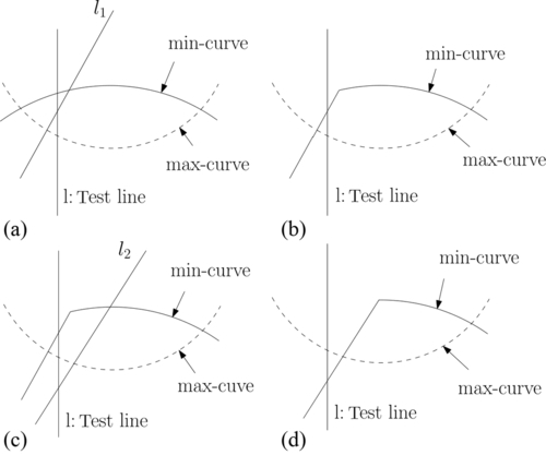
Assume that after i iterations, we determined that the minimum lies in the interval [u1, u2]. Let us see how to prune redundant constraints from the set of constraints that determine the min-curve. We make an arbitrary pairing of the bounding lines of these constraints. With respect to the interval [u1, u2], the intersection of such a constraint pair can lie as shown in Figure 12.3(a). For the ones that lie to the left (right) of the line ![]() , we prune the constraint whose bounding line has a larger (smaller) slope. Likewise, we can prune redundant constraints from the set of constraints that determine the max-curve.
, we prune the constraint whose bounding line has a larger (smaller) slope. Likewise, we can prune redundant constraints from the set of constraints that determine the max-curve.

In order to further narrow down the interval on the u-axis where the minimum lies, for all other pairs of constraints whose intersections lie within the interval [u1, u2], we find the median umed of the u-coordinates of the intersections and let ![]() be the line with respect to which we test for the location of the minimum. We make this test by examining the intersections of the min-curve and max-curve with l. This is accomplished by using the residual constraint sets that implicitly define the min-curve and max-curve. From the relative positions of these intersections and the slopes of the bounding lines of the constraints that determine these intersections, we can determine on which side of l, the minimum lies (see Figure 12.3(b)). Next, we prune a constraint from each pair whose intersections lie within [u1, u2] but on the side opposite to which the minimum lies. Because of our choice of the test-line, we are guaranteed to throw a quarter of the constraints from those that determine these intersections. We now reset the interval that contains the minimum to [umed, u2] or [u1, umed].
be the line with respect to which we test for the location of the minimum. We make this test by examining the intersections of the min-curve and max-curve with l. This is accomplished by using the residual constraint sets that implicitly define the min-curve and max-curve. From the relative positions of these intersections and the slopes of the bounding lines of the constraints that determine these intersections, we can determine on which side of l, the minimum lies (see Figure 12.3(b)). Next, we prune a constraint from each pair whose intersections lie within [u1, u2] but on the side opposite to which the minimum lies. Because of our choice of the test-line, we are guaranteed to throw a quarter of the constraints from those that determine these intersections. We now reset the interval that contains the minimum to [umed, u2] or [u1, umed].
This algorithm allows us to determine feasibility as soon as we have found a test line such that the intersection of the min-curve with l lies above its intersection with the max-curve. We implemented this offline algorithm both in two and three dimensions from scratch. Ours is probably the first such implementation in three dimensions. Refer to Megiddo (1984) for details.
Offline algorithms are effective for determining linear separability. However, as most of the gene-pairs and gene-triplets are not linearly separating, incremental algorithms would be more efficient than offline ones. This was also observed by Unger and Chor (2010). In view of this fact, in the next section, we discuss in detail an incremental version of this algorithm.
4 Incremental approach
The following obvious but useful theorem (which is true in any dimension ![]() ) underlies our algorithm in dual space:
) underlies our algorithm in dual space:
Theorem 12.1
Let ![]() and
and ![]() be arbitrary subsets of SB and SR, respectively. If
be arbitrary subsets of SB and SR, respectively. If ![]() and
and ![]() are linearly inseparable, then so are SB and SR.
are linearly inseparable, then so are SB and SR.
Proof: Straightforward: if SB and SR are linearly separable, then so are ![]() and
and ![]() .
.
4.1 Incremental approach—2D
First, we choose a small constant number of lines from each of the duals of SR and SB and use the offline approach described in the previous section to determine if there is a feasible solution to this constant-size problem. If not, we declare infeasibility (Theorem 12.1) and terminate. Otherwise, we have an initial feasible region and a test line ![]() .
.
We continued, adding a line from one of the residual sets SA* or SB*, which was also chosen randomly. Several cases can arise as a result. This line (a) becomes a part of the boundary of the feasible region, (b) leaves it unchanged, or (c) establishes infeasibility, in which case the algorithm terminates. Case (a) spawns two subcases, as shown in Figure 12.4. (a.1) the test line l still intersects the feasible region (see Figure 12.4 (a) and (b)). (a.2) the test line l goes outside the feasible region (see Figure 12.4 (c) and (d)). The lines belonging to the case (b) always leads to a condition mentioned in (a.1).
If the test line l goes outside the feasible region, constraint-pruning is triggered. This consists of examining pairs of constraints whose intersections lie on the side of l that does not include the feasible region. One of the constraints of each such pair does not intersect the feasible region and therefore is eliminated from further consideration. However, if l lies inside the new feasible interval, we continue to add new lines.
If we are able to add all lines without case (c) occurring, then we have a feasible region, and hence a separating line in the primal space.
A formal description of the iterative algorithm is as follows:
Algorithm IncrementallySeparatingGenepairs
Input: Line duals SR* and SB* of the point sets SR and SB.
Output: LP feasible or infeasible.
1: Choose ![]() and
and ![]() so that
so that ![]() .
.
2: Apply the offline approach to ![]() and
and ![]() . We have the following cases:
. We have the following cases:
Case 1: If infeasible, then report this and halt.
Case 2: If feasible, then return the vertical test line l and continue with step 3.
3: Repeatedly add a line from ![]() or
or ![]() until no more lines remain to be added or there exists no feasible point on the test line l.
until no more lines remain to be added or there exists no feasible point on the test line l.
4: If there is a feasible point on the test line l we report separability and halt.
5: If there is no feasible point on the test line l, determine on which side of l the feasible solution lies.
6: Update ![]() and
and ![]() by eliminating a line from each pair whose intersection does not lie in the feasible region and was earlier used to determine l.
by eliminating a line from each pair whose intersection does not lie in the feasible region and was earlier used to determine l.
7: Update ![]() and
and ![]() by including all those lines added in step 3 and go to step 2.
by including all those lines added in step 3 and go to step 2.
When SR and SB are linearly separable (LS), the running time of the incremental algorithm is linear in the total number of inputs. Otherwise, as the algorithm terminates when a line added that reveals inseparability, the time complexity for this case is linear in the number of lines added so far.
Theorem 12.2
If m is the total number of samples, then time complexity of the incremental algorithm is O(m).
Proof: In each iteration, the algorithm prunes one-quarter of the constraints (i.e., samples) from the current set ![]() . The time complexity of each iteration is O(m). The run time T(m) satisfies the recurrence
. The time complexity of each iteration is O(m). The run time T(m) satisfies the recurrence ![]() , whose solution is
, whose solution is ![]() .
.
4.2 Incremental approach—3D
Suppose that constraints (i.e., planes) belong to a three-dimensional (3D) Cartesian coordinate system with axes labeled as U, V, and Z, and the position of any point in 3D space is given by an ordered triple of real numbers (u1, u2, u3). These numbers give the distance of that point from the origin measured along the axes.
First, we applied a 3D offline approach on a small constant number of constraints (i.e., planes) from each dual of SR and SB. If this constant size problem is infeasible, then we report infeasibility and terminate (see Theorem 12.1). Otherwise, we have a vertical test plane that passes through the feasible region. This vertical test plane is parallel to either the VZ-plane (say ![]() ) or the UZ-plane (say
) or the UZ-plane (say ![]() ) and chosen suitably, as suggested by Megiddo.
) and chosen suitably, as suggested by Megiddo.
A formal description of the iterative algorithm is as follows:
Algorithm IncrementalySeparatingGeneTriplets
Input: Plane duals SR* and SB* of the point sets SR and SB.
Output: LP feasible or infeasible.
1: Initialize ![]() and
and ![]() . We can choose
. We can choose ![]() .
.
2: Apply Megiddo’s approach to ![]() and
and ![]() . We have the following cases:
. We have the following cases:
Case 1: If infeasible, then report the inseparability and halt.
Case 2: If feasible, then return a vertical test plane Ū (or ![]() ) and continue with step 3.
) and continue with step 3.
3: Repeatedly add a constraint from ![]() or
or ![]() and initiate an incremental 2-D approach on vertical test plane Ū (or
and initiate an incremental 2-D approach on vertical test plane Ū (or ![]() ). We distinguish with following cases:
). We distinguish with following cases:
Case 1: If the test plane Ū (or ![]() ) is feasible after all the constraints are considered, then report separability and halt.
) is feasible after all the constraints are considered, then report separability and halt.
Case 2: If the test plane Ū (or ![]() ) is infeasible, then solve two 2D linear programs to determine on which side of test plane the feasible region lies.
) is infeasible, then solve two 2D linear programs to determine on which side of test plane the feasible region lies.
Case 2.1: If any one of 2D linear program is feasible, then identify the side of feasible solution and continue with step 4.
Case 2.2: If both 2D linear program are not feasible or both are feasible, then report the inseparability and halt.
4: Identify a second vertical test plane ![]() (or Ū) and initiate an incremental 2D approach by resuming the addition of constraints from
(or Ū) and initiate an incremental 2D approach by resuming the addition of constraints from ![]() or
or ![]() , excluding those which are already being considered with Ū (or
, excluding those which are already being considered with Ū (or ![]() ). If we do not have any second vertical test plane, then continue with step 5. We distinguish with the following cases:
). If we do not have any second vertical test plane, then continue with step 5. We distinguish with the following cases:
Case 1: If the test plane ![]() (or Ū) is feasible after all the constraints are considered, then report separability and halt.
(or Ū) is feasible after all the constraints are considered, then report separability and halt.
Case 2: If the test plane ![]() (or Ū) is infeasible, then solve two 2D linear programs to determine on which side of test plane the feasible region lies.
(or Ū) is infeasible, then solve two 2D linear programs to determine on which side of test plane the feasible region lies.
Case 2.1: If any one of 2D linear program is feasible, then identify the side of feasible solution and continue with step 5.
Case 2.2: If both 2D linear program are not feasible or both are feasible, then report the inseparability and halt.
5: Update ![]() and
and ![]() by eliminating a constraint from each coupled line which does not pass through the feasible quadrant Ū and
by eliminating a constraint from each coupled line which does not pass through the feasible quadrant Ū and ![]() .
.
6: Update ![]() and
and ![]() by including all those constraints considered in step 3 and step 4.
by including all those constraints considered in step 3 and step 4.
7: Repeat the algorithm for the updated set of ![]() and
and ![]() .
.
4.3 Linear programming formulation of Unger and Chor’s incremental algorithm
Unger and Chor (2010) proposed an incremental algorithm for testing separability with respect to gene pairs. They considered m1. m2 vectors obtained by joining every point in the class SR (or SB) to every point of the class SB (or SR) (see Figure 12.5). The directions corresponding to these vectors map to m1. m2 points on a unit circle, with the center at O. In this formulation, the sample classes SR and SB are LS if the points on the unit circle span arc are less than π.


We can reformulate this in our linear programming framework. Let ![]() be the coordinates of the points corresponding to all the directions on the perimeter of the unit circle. We make the following observation:
be the coordinates of the points corresponding to all the directions on the perimeter of the unit circle. We make the following observation:
Observation. The points ![]() , span an angle less than π if there exists a line, l, through O such that all the points lie on one side of it.
, span an angle less than π if there exists a line, l, through O such that all the points lie on one side of it.
maximize/minimize u
or
maximize/minimize u
We summarize this discussion with the following claims:
Claim 1. If ![]() , then l*(u, 0) is a point in a dual plane such that it is either above or below of all the lines
, then l*(u, 0) is a point in a dual plane such that it is either above or below of all the lines ![]() .
.
Equivalently,
Claim 2. If ![]() , then
, then ![]() is a line in a primal plane such that all the points
is a line in a primal plane such that all the points ![]() lie on one side of this line.
lie on one side of this line.
The incremental implementation based on the abovementioned LP formulation is as simple as the one in Unger and Chor (2010), and it also provides early termination when inseparability is detected. In the worst case, the running time of both formulations is quadratic in the sample size m.
5 Gene selection
Gene selection is an important preprocessing step for the classification of the gene expression data set. This helps (a) to reduce the size of the gene expression data set and improve classification accuracy; (b) to cut down the presence of noise in the gene expression data set by identifying informative genes; and (c) to improve the computation by removing irrelevant genes that not only add to the computation time, but also make classification harder.
5.1 Background
In this subsection, we briefly discuss some popular score functions used for gene selection and compare them with our gene selection method, proposed in the next section. A simple approach to feature selection is to use the correlation between gene expression values and class labels. This method was first proposed by Golub et al. (1999). The correlation metric defined by Nguyen and Rocke (2002) and by Golub et al. reflects the difference between the class mean relative to standard deviation within the class. The high absolute value of this correlation metric favors those genes that are highly expressed in one class as compared to the other class, while their sign indicates the class in which the gene is highly expressed. We have chosen to select genes based on a t-statistic defined by Nguyen and Rocke.
For the ith gene, a t-value is computed using the following formula:

where nk, μki, and σki2 are the sample size, mean, and variance of the ith gene, respectively, of class ![]() .
.
Another important feature selection method is based on the Fisher score (Bishop, 1995; Zhang et al., 2008). The Fisher score criterion (FCS) for the ith gene can be defined as

where nk, μki, and σki2 are the sample size, mean, and variance of the ith gene, respectively, of class ![]() and μi represents the mean of the ith gene.
and μi represents the mean of the ith gene.
Significance analysis of microarrays (SAM) proposed by Tusher et al. (2001) is another important gene filter technique for finding significant genes in a set of microarray experiments. The SAM score for each gene can be defined as
For simplicity, the correcting constant s0 is set to 1 and si is computed as follows:

where xji is the jth sample of the ith gene. The classes 1 and 2 are represented by C1 and C2. Similarly, nk, μki, and σki2 are the sample size, mean, and variance of the ith gene, respectively, of class ![]() .
.
For the purpose of generating significant genes by SAM, we have used software written by Chu et al. (2001), which is publicly available at http://www-stat.stanford.edu/tibs/clickwrap/sam/academic.
6 A new methodology for gene selection
To find a set of genes that are large enough to be robust against noise and small enough to be applied to the clinical setting, we propose a simple gene selection strategy based on an individual gene-ranking approach. This consists of two steps: coarse filtration, followed by fine filtration.
6.1 Coarse filtration
The purpose of coarse filtration is to remove most of the attributes that contribute to noise in the gene expression data set. This noise can be categorized into (i) biological noise and (ii) technical noise (Lu and Han, 2003). Biological noise refers to the genes in a gene expression data set that are irrelevant for classification. Technical noise refers to errors incurred at various stages during data preparation.
For coarse filtration, we follow an established approach based upon the t-metric discussed in the previous section. Following a general consensus (Golub et al., 1999; Kim et al., 2002), we chose to select a sufficient number of genes that can be further considered for fine filtration. This is a set of 100 genes obtained by taking 50 genes with the largest positive t-values and another 50 genes with the smallest negative t-values.
6.2 Fine filtration
One of the problems with the abovementioned correlation metric is that the t-value is calculated from the expression values of a single gene, ignoring the information available from the other genes. To rectify this, we propose the following scheme:
Let the set of genes ![]() be the output of the coarse filtration step, where n = 100. For a gene
be the output of the coarse filtration step, where n = 100. For a gene ![]() , let
, let ![]() is an LS pair,
is an LS pair, ![]() and
and ![]() . In other words, Si consists of all genes that form LS pairs with gi. For each gene
. In other words, Si consists of all genes that form LS pairs with gi. For each gene ![]() , its Pi-value is set as
, its Pi-value is set as ![]() .
.
The intuition underlying this definition is that the informative genes have very different expression values in the two classes. If such genes exist in the gene expression data set, then this ranking strategy will assign the highest rank to those genes.
A drawback of this gene selection method is that it is applicable only to those gene expression data sets that have LS pairs. For those data sets that have few LS pairs, such as Lung Cancer (Gordon et al., 2002) and Breast Cancer (van’t Veer et al., 2002), we can extend the definition using LS gene triplets:
For a gene ![]() , set
, set
In other words, Qi consists of all gene pairs (gj, gk) that make up an LS triplet with the gene gi. For each gene ![]() , define
, define ![]() . Clearly, Ti lies between 0 and
. Clearly, Ti lies between 0 and ![]() .
.
7 Results and discussion
In this chapter, we have developed offline and incremental geometric tools to test linear separability of pairs and triplets of genes, followed by a simple gene selection strategy that uses these tools to rank the genes. Based upon this ranking, we chose a suitable number of top-scoring genes for a good classifier.
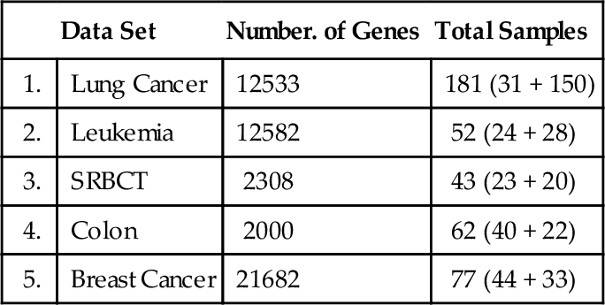
We demonstrated the usefulness of the proposed methodology by testing it against five publicly available gene expression data sets: (a) Lung Cancer (Gordon et al., 2002); (b) Leukemia (Armstrong et al., 2002); (c) SRBCT (Khan et al., 2001); (d) Colon (Alon et al., 1999); and (e) Breast Cancer (van’t Veer et al., 2002). Table 12.1 shows the number of samples in each data set, with the number of samples from each class in parentheses.
Table 12.1
Five Gene Expression Data Sets
| Data Set | Number. of Genes | Total Samples | |
| 1. | Lung Cancer | 12533 | 181 (31 + 150) |
| 2. | Leukemia | 12582 | 52 (24 + 28) |
| 3. | SRBCT | 2308 | 43 (23 + 20) |
| 4. | Colon | 2000 | 62 (40 + 22) |
| 5. | Breast Cancer | 21682 | 77 (44 + 33) |
The 100 genes that we selected from each of these data sets in the Coarse Filtration step effectively prunes away most of the attributes (genes) that are irrelevant for classification. On the other hand, this number is large enough to provide us with a number of attributes (genes) that may be overfitting for classifier construction.
To get the best subset of genes for good classification, we chose to populate the attribute space with 5, 10, 15, 25, and 30 genes from each data set by applying Fine Filtration. The choices of these attribute/feature-space sizes are somewhat arbitrary, but the chosen attribute/feature spaces are sufficiently large in comparison to the size of the sample spaces, as Table 12.1 shows.
The computational time of the Fine Filtration step depends upon the geometric tool that we use to check the separability of gene expression data. In this chapter, we have presented linear, time-incremental algorithms for both gene pairs and gene triplets. In order to illustrate the effectiveness of this approach, we ran both versions (offline and incremental) on each of the five data sets obtained by Coarse Filtration. The computing platform was a Dell Inspiron 1545 model–Intel Core2 Duo central processing unit (CPU), 2.00 GHz, and 2 GB RAM, running under Microsoft Windows Vista. The run-time efficiency of the incremental version over the offline one is evident from Table 12.2.
Table 12.2
2D and 3D Separability Test with Run Time
| 2D Separability Test with RT | 3D Separability Test with RT | |||||||
| Data Set | LSP (%) | RT of Offline (ms) | RT of Incr. (ms) | Impr. of Incr. over Offline (%) | PLST (%) | RT of Offline (ms) | RT of Incr. (ms) | Impr. of Incr. over Offline (%) |
| Lung Cancer | 0.72 | 4617 | 1537 | 66.71 | 0.946 | 1114467 | 166662 | 85.04 |
| Leukemia | 11.92 | 1138 | 418 | 63.27 | 3.72 | 115791 | 49263 | 57.45 |
| SRBCT | 8.86 | 987 | 356 | 63.93 | 4.11 | 92825 | 52080 | 43.89 |
| Colon | 0 | 1328 | 275 | 79.29 | 0 | 170143 | 39955 | 76.516 |
| Breast Cancer | 0.93 | 1606 | 440 | 72.6 | 0.137 | 274141 | 83913 | 69.39 |

Note: RT: run time, Incr.: incremental, Impr.: improvement.
A group of genes that is being tested for linear separability may include a gene that is a perfect one-dimensional (1D) separator with a TNoM score of zero, using the terminology of Ben-Dor et al. (2000). In this case, such a group will provide a positive separability test. In order to exclude such groups, we checked for the existence of such 1D separators and found that no such genes exists in these data sets. Likewise, if a gene pair shows linear separability, then all gene triplets that include these gene pairs will also be linearly separating. In order to count gene triplets that exhibit pure 3D linear separability, we avoided testing gene triplets that included an LS pair. Thus, our 3D test results shown here include only such gene triplets. We call such gene triplets Perfect Linearly Separable Triplet (PLSTs). The percentage of Linearly Separable Pairs (LSPs), Linearly Separable Triplets (LSTs), and Perfect Linearly Separable Triplets (PLSTs) are calculated using these formulas:


where n is the total number of genes in the gene expression data set.
These formulas show that the total number of triplets relative to the PLSTs is much higher than the total number of pairs relative to the LSPs. Thus, the increase in the actual number of PLSTs over the number of LSPs is suppressed by the high value of the denominator in the former case. The separability test shows that Colon (Alon et al., 1999) data set has neither any LSPs nor any PLSTs. The Lung Cancer (Gordon et al., 2002) and Breast Cancer (van’t Veer et al., 2002) data sets have a few LSPs, whereas the number of PLSTs is 41 and 5 times (approximately) the number of LSPs, respectively. The Leukemia (Armstrong et al., 2002) and SRBCT (Khan et al., 2001) data sets show a good number of LSPs, while the number of PLSTs is 6 and 11 times (approximately) the number of LSPs, respectively.
The motive underlying our gene selection strategy is to identify if a gene, jointly with other genes, has the class distinction property. In the current study, we identified the class distinction property by separability tests where the group size was restricted to pairs and triplets. As the Colon data set (Alon et al., 1999) did not show any positive separability result, we continued our study with the remaining four gene expression data sets. This result in Colon is not surprising at all, since according to Alon et al. (1999), some samples such as T2, T30, T33, T36, T37, N8, N12, and N34 have been identified as outliers and presented with an anomalous muscle-index. This confirms the uncertainty of these samples.
Next, in the Fine Filtration stage, we used the incremental version of our algorithm to test separability by gene pairs and assign a Pi value to a gene ![]() . Based on the ranking, we chose a set of top-scoring genes to populate five different feature spaces of size 5, 10, 15, 20, 25, and 30. If more than one gene had the same rank, then we chose an arbitrary gene from that peer group. To compare our method with other selection methods, such as t-metric, FCS, and SAM, we populated similar feature spaces respectively.
. Based on the ranking, we chose a set of top-scoring genes to populate five different feature spaces of size 5, 10, 15, 20, 25, and 30. If more than one gene had the same rank, then we chose an arbitrary gene from that peer group. To compare our method with other selection methods, such as t-metric, FCS, and SAM, we populated similar feature spaces respectively.
For classification, we used machine learning (ML) tools supported by WEKA version 3.6.3 (Hall et al., 2009). We used the following two classifiers:
1. Support Vector Classifier: WEKA SMO class implements John C. Platt’s (Platt, 1998) sequential minimal optimization algorithm for training a support vector classifier. We used a linear kernel.
2. Bayes Network Classifier: The Weka BayesNet class implements Bayes network learning using various search algorithms and quality measures (Bouckaert, 2004).
We chose the Bayes Network classifier based on K2 for learning structure (Cooper and Herskovits, 1992). Both of these classifiers normalized the attributes by default to provide a better classification result. We used a 10-fold cross-validation (Kohavi, 1995) for prediction, as shown in Figure 12.6. As suggested (Kohavi, 1995), we have used 10-fold stratified cross-validation. In stratified cross-validation, the folds are stratified so that they contain approximately the same proportions of labels as original data sets.

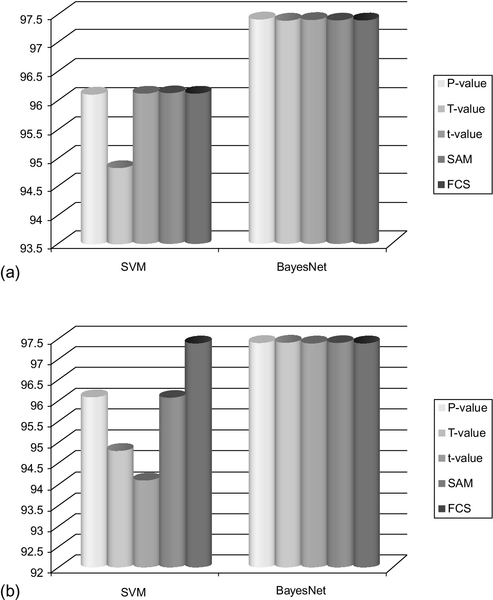
A comparative classification accuracy of the feature spaces generated from P-values, t-values, FCS, and SAM is shown in Figures 12.7–12.10. The results clearly show that the gene spaces generated by P-values yield a good classifier. Specifically, the feature spaces of sizes 10, 15, 20, 25, and 30 generated by the P-values perform mostly as well as or better than the feature spaces generated by the t-values, FCS and SAM.


To illustrate the performance of the classifiers with respect to the feature spaces generated by the T-values, we considered two data sets with few LSPs, such as Lung Cancer (Gordon et al., 2002) and Breast Cancer (van’t Veer et al., 2002). To make sure that the data set has no LSPs, we removed all genes that are responsible for pair separability in the selection process. Then feature spaces of size 5, 10, 15, 20, 25, and 30 were populated based upon the T-values. The classification results are shown in Figures 12.7–12.10. It is interesting to note that the feature space generated from Lung Cancer (Gordon et al., 2002) data set by T-values achieves similar or even better classification accuracy compared to t-values, FCS and SAM. In Figures 12.11–12.14, we have shown the classification accuracy of feature space confined to 25 and 30.


8 Conclusions
Our empirical study of the four data sets discussed in this chapter shows that the feature space generated by our methods (particularly by the use of P-values) is as good as the feature selection methods based on t-values, SAM, and FCS. Toward the broader objective of identifying important biomarkers to distinguish between input classes, we list in Table 12.3 the top 10 genes (or genes attached to a probe set in the respective microarray experiments) from each of the data sets.
Table 3
Top ten significant genes based upon P-values
| Dataset | Probe Set or Image | Gene Name or Description |
| Leukemia Data | 39318_at | Hs.2484 gnl|UG|Hs#S4305 H.sapiens mRNA for Tcell leukemia |
| 36571_at | Hs.75248 gnl|UG|Hs#S5526 H.sapiens topIIb mRNA for topoisomerase IIb | |
| 41462_at | Hs.11183 gnl|UG|Hs#S1055230 H.sapiens sorting nexin 2 (SNX2) mRNA, complete cds | |
| 266_s_at | M26692 /FEATURE=exon#1 /DEFINITION=HUMLCKPR02 Homo sapiens lymphocyte-specific protein tyrosine kinase (LCK) gene, exon 1, and downstream promoter region | |
| 34168_at | Hs.272537 gnl|UG|Hs#S1611 Human terminal transferase mRNA, complete cds | |
| 40285_at | Hs.58927 gnl|UG|Hs#S876152 Homo sapiens nuclear VCP-like protein NVLp.2 (NVL.2) mRNA, complete cds | |
| 40533_at | Hs.1578 gnl|UG|Hs#S1266737 tg78b04.x1 Homo sapiens cDNA, 3' end | |
| 38017_at | Hs.79630 gnl|UG|Hs#S551444 Human MB-1 gene, complete cds | |
| 40282_s_at | Hs.155597 gnl|UG|Hs#S779 Human adipsin | |
| 39520_at | Hs.100729 gnl|UG|Hs#S1526847 wn60d01.x1 Homo sapiens cDNA, 3' end | |
| Lung Cancer | 33328_at | |
| 36533_at | ||
| 33833_at | ||
| 31684_at | ||
| 41388_at | ||
| 1662_r_at | ||
| 33904_at | ||
| 36105_at | ||
| 33245_at | ||
| 39756_g_at | ||
| Breast Cancer | Contig53226_RC | |
| AI147042_RC | ||
| NM_000790 | ||
| Contig1789_RC | ||
| NM_000238 | ||
| AB037821 | ||
| AB033007 | ||
| NM_000353 | ||
| NM_002073 | ||
| AF053712 | ||
| SRBCT | 770394 | Fc fragment of IgG, receptor, transporter, alpha |
| 377461 | caveolin 1, caveolae protein, 22kD | |
| 1435862 | antigen identified by monoclonal antibodies 12E7, F21 and O13 | |
| 814260 | follicular lymphoma variant translocation 1 | |
| 866702 | protein tyrosine phosphatase, non-receptor type 13 (APO-1/CD95 (Fas)-associated phosphatase) | |
| 52076 | olfactomedinrelated ER localized protein | |
| 357031 | tumor necrosis factor, alpha-induced protein 6 | |
| 43733 | glycogenin 2 | |
| 207274 | Human DNA for insulin-like growth factor II (IGF-2); exon 7 and additional ORF | |
| 898219 | mesoderm specific transcript (mouse) homolog |

We presented a gene selection strategy to achieve high classification accuracy. The gene selection strategy exploits the class-distinguishing property of genes by testing separability by pairs and triplets. To test for separability, we provided two versions of a linear time algorithm and demonstrated that the run time of the incremental version is markedly better than that of the offline version. The importance of this method lies in the fact that it can be easily extended to higher dimensions, allowing us to test if groups of more than three genes can separate the data sets. In this study, we limited the separability tests to gene pairs and triplets and used this criteria to rank the genes.