Chapter 10. Scalar Optimizations
An optimizing compiler improves the quality of the code that it generates by applying transformations that rewrite the code. This chapter builds on the introduction to optimization provided in Chapter 8 and the material on static analysis in Chapter 9 to focus on optimization of the code for a single thread of control—so-called scalar optimization. The chapter introduces a broad selection of machine-independent transformations that address a variety of inefficiencies in the compiled code.
Keywords: Optimization, Transformation, Machine Dependent, Machine Independent, Redundancy, Dead Code, Constant Propagation
10.1. Introduction
An optimizer analyzes and transforms the code with the intent to improve its performance. The compiler uses static analyses, such as data-flow analysis (see Chapter 9) to discover opportunities for transformations and to prove their safety. These analyses are preludes to transformations—unless the compiler rewrites the code, nothing will change.
Code optimization has a history that is as long as the history of compilers. The first
fortran compiler included careful optimization with the intent to provide performance that rivaled hand-coded assembly code. Since that first optimizing compiler in the late 1950s, the literature on optimization has grown to include thousands of papers that describe analyses and transformations.
Deciding which transformations to use and selecting an order of application for them remains one of the most daunting decisions that a compiler writer faces. This chapter focuses on
scalar optimization, that is, optimization of code along a single thread of control. It identifies five key sources of inefficiency in compiled code and then presents a set of optimizations that help to remove those inefficiencies. The chapter is organized around these five effects; we expect that a compiler writer choosing optimizations might use the same organizational scheme.
Scalar Optimization
code improvement techniques that focus on a single thread of control
Conceptual Roadmap
Compiler-based optimization is the process of analyzing the code to determine its properties and using the results of that analysis to rewrite the code into a more efficient or more effective form. Such improvement can be measured in many ways, including decreased running time, smaller code size, or lower processor energy use during execution. Every compiler has some set of input programs for which it produces highly efficient code. A good optimizer should make that performance available on a much larger set of inputs. The optimizer should be robust, that is, small changes in the input should not produce wild performance changes.
An optimizer achieves these goals through two primary mechanisms. It eliminates unnecessary overhead introduced by programming language abstractions and it matches the needs of the resulting program to the available hardware and software resources of the target machine. In the broadest sense, transformations can be classified as either
machine independent or
machine dependent. For example, replacing a redundant computation with a reuse of the previously computed value is usually faster than recomputing the value; thus, redundancy elimination is considered machine independent. By contrast, implementing a character string copy operation with the “scatter-gather” hardware on a vector processor is clearly
machine dependent. Rewriting that copy operation with a call to the hand-optimized system routine
bcopy might be more broadly applicable.
Machine Independent
A transformation that improves code on most target machines is considered
machine independent.
Machine Dependent
A transformation that relies on knowledge of the target processor is considered
machine dependent.
 |
Overview
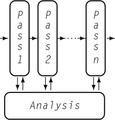
Most optimizers are built as a series of passes, as shown in the margin. Each pass takes code in
Ir form as its input. Each pass produces a rewritten version of the
Ir code as its output. This structure breaks the implementation into smaller pieces and avoids some of the complexity that arises in large, monolithic programs. It allows the passes to be built and tested independently, which simplifies development, testing, and maintenance. It creates a natural way for the compiler to provide different levels of optimization; each level specifies a set of passes to run. The pass structure allows the compiler writer to run some passes multiple times, if desirable. In practice, some passes should run once, while others might run several times at different points in the sequence.
Optimization Sequences
The choice of specific transformations and the order of their application has a strong impact on the effectiveness of an optimizer. To make the problem harder, individual transformations have overlapping effects (e.g. local value numbering versus superlocal value numbering) and individual applications have different sets of inefficiencies.
Equally difficult, transformations that address different effects interact with one another. A given transformation can create opportunities for other transformations. Symmetrically, a given transformation can obscure or eliminate opportunities for other transformations.
Classic optimizing compilers provide several levels of optimization (e.g.
-O,
−O1,
−O2, …) as one way of providing the end user with multiple sequences that they can try. Researchers have focused on techniques to derive custom sequences for specific application codes, selecting both a set of transformations and an order of application. Section 10.7.3 discusses this problem in more depth.
In the design of an optimizer, the selection of transformations and the ordering of those transformations play a critical role in determining the overall effectiveness of the optimizer. The selection of transformations determines what specific inefficiencies in the
ir program the optimizer discovers and how it rewrites the code to reduce those inefficiencies. The order in which the compiler applies the transformations determines how the passes interact.
For example, in the appropriate context (
r
2 > 0 and
r
5 = 4), an optimizer might replace
mult r
2, r
5 ⇒ r
17 with
lshiftI r
2, 2 ⇒ r
17. This change replaces a multicycle integer multiply with a single-cycle shift operation and reduces demand for registers. In most cases, this rewrite is profitable. If, however, the next pass relies on commutativity to rearrange expressions, then replacing a multiply with a shift forecloses an opportunity (multiply is commutative, shift is not). To the extent that a transformation makes later passes less effective, it may hurt overall code quality. Deferring the replacement of multiplies by shifts may avoid this problem; the context needed to prove safety and profitability for this rewrite is likely to survive the intervening passes.
The first hurdle in the design and construction of an optimizer is conceptual. The optimization literature describes hundreds of distinct algorithms to improve
ir programs. The compiler writer must select a subset of these transformations to implement and apply. While reading the original papers may help with the implementation, it provides little insight for the decision process, since most of the papers advocate using their own transformations.
Compiler writers need to understand both what inefficiencies arise in applications translated by their compilers and what impact those inefficiencies have on the application. Given a set of specific flaws to address, they can then select specific transformations to address them. Many transformations, in fact, address multiple inefficiencies, so careful selection can reduce the number of passes needed. Since most optimizers are built with limited resources, the compiler writer can prioritize transformations by their expected impact on the final code.
As mentioned in the conceptual roadmap, transformations fall into two broad categories: machine-independent transformations and machine-dependent transformations. Examples of machine-independent transformations from earlier chapters include local value numbering, inline substitution, and constant propagation. Machine-dependent transformations often fall into the realm of code generation. Examples include peephole optimization (see Section 11.5), instruction scheduling, and register allocation. Other machine-dependent transformations fall into the realm the optimizer. Examples include tree-height balancing, global code placement, and procedure placement. Some transformations resist classification; loop unrolling can address either machine-independent issues such as loop overhead or machine-dependent issues such as instruction scheduling.
The distinction between the categories can be unclear. We call a transformation machine independent if it deliberately ignores target machine considerations, such as its impact on register allocation.
Chapter 8 and Chapter 9 have already presented a number of transformations, selected to illustrate specific points in those chapters. The next three chapters focus on code generation, a machine-dependent activity. Many of the techniques presented in these chapters, such as peephole optimization, instruction scheduling, and register allocation, are machine-dependent transformations. This chapter presents a broad selection of transformations, mostly machine-independent transformations. The transformations are organized around the effect that they have on the final code. We will concern ourselves with five specific effects.
■
Eliminate useless and unreachable code The compiler can discover that an operation is either useless or unreachable. In most cases, eliminating such operations produces faster, smaller code.
■
Move code The compiler can move an operation to a place where it executes fewer times but produces the same answer. In most cases, code motion reduces runtime. In some cases, it reduces code size.
■
Eliminate a redundant computation The compiler can prove that a value has already been computed and reuse the earlier value. In many cases, reuse costs less than recomputation. Local value numbering captures this effect.
■
Enable other transformations The compiler can rewrite the code in a way that exposes new opportunities for other transformations. Inline substitution, for example, creates opportunities for many other optimizations.
Optimization as Software Engineering
Having a separate optimizer can simplify the design and implementation of a compiler. The optimizer simplifies the front end; the front end can generate general-purpose code and ignore special cases. The optimizer simplifies the back end; the back end can focus on mapping the
IR version of the program to the target machine. Without an optimizer, both the front end and back end must be concerned with finding opportunities for improvement and exploiting them.
In a pass-structured optimizer, each pass contains a transformation and the analysis required to support it. In principle, each task that the optimizer performs can be implemented once. This provides a single point of control and lets the compiler writer implement complex functions once, rather than many times. For example, deleting an operation from the
IR can be complicated. If the deleted operation leaves a basic block empty, except for the block-ending branch or jump, then the transformation should also delete the block and reconnect the block's predecessors to its successors, as appropriate. Keeping this functionality in one place simplifies implementation, understanding, and maintenance.
From a software engineering perspective, the pass structure, with a clear separation of concerns, makes sense. It lets each pass focus on a single task. It provides a clear separation of concerns—value numbering ignores register pressure and the register allocator ignores common subexpressions. It lets the compiler writer test passes independently and thoroughly, and it simplifies fault isolation.
This set of categories covers most machine-independent effects that the compiler can address. In practice, many transformations attack effects in more than one category. Local value numbering, for example, eliminates redundant computations, specializes computations with known constant values, and uses algebraic identities to identify and remove some kinds of useless computations.
10.2. Eliminating Useless and Unreachable Code
Sometimes, programs contain computations that have no externally visible effect. If the compiler can determine that a given operation does not affect the program's results, it can eliminate the operation. Most programmers do not write such code intentionally. However, it arises in most programs as the direct result of optimization in the compiler and often from macro expansion or naive translation in the compiler's front end.
Two distinct effects can make an operation eligible for removal. The operation can be
useless, meaning that its result has no externally visible effect. Alternatively, the operation can be
unreachable, meaning that it cannot execute. If an operation falls into either category, it can be eliminated. The term
dead code is often used to mean either useless or unreachable code; we use the term to mean useless.
Useless
An operation is
useless if no operation uses its result, or if all uses of the result are, themselves dead.
Unreachable
An operation is
unreachable if no valid control-flow path contains the operation.
Removing useless or unreachable code shrinks the
ir form of the code, which leads to a smaller executable program, faster compilation, and, often, to faster execution. It may also increase the compiler's ability to improve the code. For example, unreachable code may have effects that show up in the results of static analysis and prevent the application of some transformations. In this case, removing the unreachable block may change the analysis results and allow further transformations (see, for example, sparse conditional constant propagation, or
sccp, in Section 10.7.1).
Some forms of redundancy elimination also remove useless code. For instance, local value numbering applies algebraic identities to simplify the code. Examples include
x + 0 ⇒ x, y × 1 ⇒ y, and
max(z, z) ⇒ z. Each of these simplifications eliminates a useless operation—by definition, an operation that, when removed, makes no difference in the program's externally visible behavior.
Because the algorithms in this section modify the program's control-flow graph (
cfg), we carefully distinguish between the terms
branch, as in an
iloccbr, and
jump, as in an
ilocjump. Close attention to this distinction will help the reader understand the algorithms.
10.2.1. Eliminating Useless Code
An operation can set a return value in several ways, including assignment to a call-by-reference parameter or a global variable, assignment through an ambiguous pointer, or passing a return value via a return statement.
The classic algorithms for eliminating useless code operate in a manner similar to mark-sweep garbage collectors with the
IR code as data (see Section 6.6.2). Like mark-sweep collectors, they perform two passes over the code. The first pass starts by clearing all the mark fields and marking “critical” operations as “useful.” An operation is
critical if it sets return values for the procedure, it is an input/output statement, or it affects the value in a storage location that may be accessible from outside the current procedure. Examples of critical operations include a procedure's prologue and epilogue code and the precall and postreturn sequences at calls. Next, the algorithm traces the operands of useful operations back to their definitions and marks those operations as useful. This process continues, in a simple worklist iterative scheme, until no more operations can be marked as useful. The second pass walks the code and removes any operation not marked as useful.
Figure 10.1 makes these ideas concrete. The algorithm, which we call
Dead, assumes that the code is in
ssa form.
ssa simplifies the process because each use refers to a single definition.
Dead consists of two passes. The first, called
Mark, discovers the set of useful operations. The second, called
Sweep, removes useless operations.
Mark relies on reverse dominance frontiers, which derive from the dominance frontiers used in the
ssa construction (see Section 9.3.2).
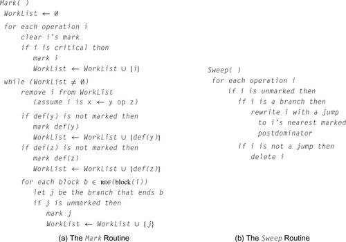
The treatment of operations other than branches or jumps is straightforward. The marking phase determines whether an operation is useful. The sweep phase removes operations that have not been marked as useful.
The treatment of control-flow operations is more complex. Every jump is considered useful. Branches are considered useful only if the execution of a useful operation depends on their presence. As the marking phase discovers useful operations, it also marks the appropriate branches as useful. To map from a marked operation to the branches that it makes useful, the algorithm relies on the notion of control dependence.
The definition of control dependence relies on
postdominance. In a
cfg, node
j postdominates node
i if every path from
i to the
cfg's exit node passes through
j. Using postdominance, we can define control dependence as follows: in a
cfg, node
j is control-dependent on node
i if and only if
1. There exists a nonnull path from
i to
j such that
j postdominates every node on the path after
i. Once execution begins on this path, it must flow through
j to reach the
cfg's exit (from the definition of postdominance).
2.
j does not strictly postdominate
i. Another edge leaves
i and control may flow along a path to a node not on the path to
j. There must be a path beginning with this edge that leads to the
cfg's exit without passing through
j.
Postdominance
In a
cfg,
j postdominates i if and only if every path from
i to the exit node passes through
j.
See also the definition of dominance on page 478.
In other words, two or more edges leave block
i. One or more edges leads to
j and one or more edges do not. Thus, the decision made at the branch-ending block
i can determine whether or not
j executes. If an operation in
j is useful, then the branch that ends
i is also useful.
This notion of control dependence is captured precisely by the
reverse dominance frontier of
j, denoted
rdf(
j). Reverse dominance frontiers are simply dominance frontiers computed on the reverse
cfg. When
Mark marks an operation in block
b as useful, it visits every block in
b's reverse dominance frontier and marks their block-ending branches as useful. As it marks these branches, it adds them to the worklist. It halts when that worklist is empty.
Sweep replaces any unmarked branch with a jump to its first postdominator that contains a marked operation. If the branch is unmarked, then its successors, down to its immediate postdominator, contain no useful operations. (Otherwise, when those operations were marked, the branch would have been marked.) A similar argument applies if the immediate postdominator contains no marked operations. To find the nearest useful postdominator, the algorithm can walk up the postdominator tree until it finds a block that contains a useful operation. Since, by definition, the exit block is useful, this search must terminate.
10.2.2. Eliminating Useless Control Flow
Optimization can change the
ir form of the program so that it has useless control flow. If the compiler includes optimizations that can produce useless control flow as a side effect, then it should include a pass that simplifies the
cfg by eliminating useless control flow. This section presents a simple algorithm called
Clean that handles this task.
Clean operates directly on the procedure's
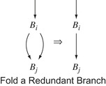
cfg. It uses four transformations, shown in the margin. They are applied in the following order:
1.
Fold a Redundant Branch If
Clean finds a block that ends in a branch, and both sides of the branch target the same block, it replaces the branch with a jump to the target block. This situation arises as the result of other simplifications. For example,
B
i might have had two successors, each with a jump to
B
j. If another transformation had already emptied those blocks, then empty-block removal, discussed next, might produce the initial graph shown in the margin.
 |
2.
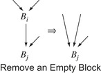
Remove an Empty Block If
Clean finds a block that contains only a jump, it can merge the block into its successor. This situation arises when other passes remove all of the operations from a block
B
i. Consider the left graph of the pair shown in the margin. Since
B
i has only one successor,
B
j, the transformation retargets the edges that enter
B
i to
B
j and deletes
B
i from
B
j's set of predecessors. This simplifies the graph. It should also speed up execution. In the original graph, the paths through
B
i needed two control-flow operations to reach
B
j. In the transformed graph, those paths use one operation to reach
B
j.
 |
3.
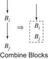
Combine Blocks If
Clean finds a block
B
i that ends in a jump to
B
j and
B
j has only one predecessor, it can combine the two blocks, as shown in the margin. This situation can arise in several ways. Another transformation might eliminate other edges that entered
B
j, or
B
i and
B
j might be the result of folding a redundant branch (described previously). In either case, the two blocks can be combined into a single block. This eliminates the jump at the end of
B
i.
 |
4.
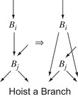
Hoist a Branch If
Clean finds a block
B
i that ends with a jump to an empty block
B
j and
B
j ends with a branch,
Clean can replace the block-ending jump in
B
i with a copy of the branch from
B
j. In effect, this hoists the branch into
B
i, as shown in the margin. This situation arises when other passes eliminate the operations in
B
j, leaving a jump to a branch. The transformed code achieves the same effect with just a branch. This adds an edge to the
cfg. Notice that
B
i cannot be empty, or else empty block removal would have eliminated it. Similarly,
B
i cannot be
B
j's sole predecessor, or else
Clean would have combined the two blocks. (After hoisting,
B
j still has at least one predecessor.)
 |
Some bookkeeping is required to implement these transformations. Some of the modifications are trivial. To fold a redundant branch in a program represented with
iloc and a graphical
cfg,
Clean simply overwrites the block-ending branch with a jump and adjusts the successor and predecessor lists of the blocks. Others are more difficult. Merging two blocks may involve allocating space for the merged block, copying the operations into the new block, adjusting the predecessor and successor lists of the new block and its neighbors in the
cfg, and discarding the two original blocks.
Many compilers and assemblers have included an ad hoc pass that eliminates a jump to a jump or a jump to a branch.
Clean achieves the same effect in a systematic way.
Clean applies these four transformations in a systematic fashion. It traverses the graph in postorder, so that
B
i's successors are simplified before
B
i, unless the successor lies along a back edge with respect to the postorder numbering. In that case,
Clean will visit the predecessor before the successor. This is unavoidable in a cyclic graph. Simplifying successors before predecessors reduces the number of times that the implementation must move some edges.
In some situations, more than one of the transformations may apply. Careful analysis of the various cases leads to the order shown in Figure 10.2, which corresponds to the order in which they are presented in this section. The algorithm uses a series of
if statements rather than an
if-then-else to let it apply multiple transformations in a single visit to a block.
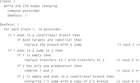
If the
cfg contains back edges, then a pass of
Clean may create additional opportunities—namely, unprocessed successors along the back edges. These, in turn, may create other opportunities. For this reason,
Clean repeats the transformation sequence iteratively until the
cfg stops changing. It must compute a new postorder numbering between calls to
OnePass because each pass changes the underlying graph. Figure 10.2 shows pseudo-code for
Clean.
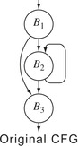 |
Clean cannot, by itself, eliminate an empty loop. Consider the
cfg shown in the margin. Assume that block
B2 is empty. None of
Clean's transformations can eliminate
B2 because the branch that ends
B2 is not redundant.
B2 does not end with a jump, so
Clean cannot combine it with
B3. Its predecessor ends with a branch rather than a jump, so
Clean can neither combine
B2 with
B1 nor fold its branch into
B1.
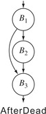 |
However, cooperation between
Clean and
Dead can eliminate the empty loop.
Dead used control dependence to mark useful branches. If
B1 and
B3 contain useful operations, but
B2 does not, then the
Mark pass in
Dead will decide that the branch ending
B2 is not useful because
B2 ∉
rdf(
B3). Because the branch is useless, the code that computes the branch condition is also useless. Thus,
Dead eliminates all of the operations in
B2 and converts the branch that ends it into a jump to its closest useful postdominator,
B3. This eliminates the original loop and produces the
cfg labelled “After Dead” in the margin.
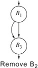 |
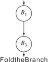
In this form,
Clean folds
B2 into
B1, to produce the
cfg labelled “Remove
B2” in the margin. This action also makes the branch at the end of
B1 redundant.
Clean rewrites it with a jump, producing the
cfg labelled “Fold the Branch” in the margin. At this point, if
B1 is
B3's sole remaining predecessor,
Clean coalesces the two blocks into a single block.
 |
This cooperation is simpler and more effective than adding a transformation to
Clean that handles empty loops. Such a transformation might recognize a branch from
Bi to itself and, for an empty
Bi, rewrite it with a jump to the branch's other target. The problem lies in determining when
Bi is truly empty. If
Bi contains no operations other than the branch, then the code that computes the branch condition must lie outside the loop. Thus, the transformation is safe only if the self-loop never executes. Reasoning about the number of executions of the self-loop requires knowledge about the runtime value of the comparison, a task that is, in general, beyond a compiler's ability. If the block contains operations, but only operations that control the branch, then the transformation would need to recognize the situation with pattern matching. In either case, this new transformation would be more complex than the four included in
Clean. Relying on the combination of
Dead and
Clean achieves the appropriate result in a simpler, more modular fashion.
10.2.3. Eliminating Unreachable Code
Sometimes the
cfg contains code that is unreachable. The compiler should find unreachable blocks and remove them. A block can be unreachable for two distinct reasons: there may be no path through the
cfg that leads to the block, or the paths that reach the block may not be executable—for example, guarded by a condition that always evaluates to false.
If the source language allows arithmetic on code pointers or labels, the compiler must preserve all blocks. Otherwise, it can limit the preserved set to blocks whose labels are referenced.
The former case is easy to handle. The compiler can perform a simple mark-sweep-style reachability analysis on the
cfg. First, it initializes a mark on each block to the value “unreachable.” Next, it starts with the entry and marks each
cfg node that it can reach as “reachable.” If all branches and jumps are unambiguous, then all unmarked blocks can be deleted. With ambiguous branches or jumps, the compiler must preserve any block that the branch or jump can reach. This analysis is simple and inexpensive. It can be done during traversals of the
cfg for other purposes or during
cfg construction itself.
Handling the second case is harder. It requires the compiler to reason about the values of expressions that control branches. Section 10.7.1 presents an algorithm that finds some blocks that are unreachable because the paths leading to them are not executable.
Section Review
Code transformations often create useless or unreachable code. To determine precisely which operations are dead, however, requires global analysis. Many transformations simply leave the dead operations in the
IR form of the code and rely on separate, specialized transformations, such as
Dead and
Clean, to remove them. Thus, most optimizing compilers include a set of transformations to excise dead code. Often, these passes run several times during the transformation sequence.
The three transformations presented in this chapter perform a thorough job of eliminating useless and unreachable code. The underlying analysis, however, can limit the ability of these transformations to prove that code is dead. The use of pointer-based values can prevent the compiler from determining that a value is unused. Conditional branches can occur in places where the compiler cannot detect the fact that they always take the same path; Section 10.8 presents an algorithm that partially addresses this problem.
Review Questions
1. Experienced programmers often question the need for useless code elimination. They seem certain that they do not write code that is useless or unreachable. What transformations from Chapter 8 might create useless code?
2. How might the compiler, or the linker, detect and eliminate unreachable procedures? What benefits might accrue from using your technique?
Hint: Write down the code to access
A[i, j] where
A is dimensioned
A[1:N, 1:M].
10.3. Code Motion
Moving a computation to a point where it executes less frequently than it executed in its original position should reduce the total operation count of the running program. The first transformation presented in this section,
lazy code motion, uses code motion to speed up execution. Because loops tend to execute many more times than the code that surrounds them, much of the work in this area has focused on moving loop-invariant expressions out of loops. Lazy code motion performs loop-invariant code motion. It extends the notions originally formulated in the available expressions data-flow problem to include operations that are redundant along some, but not all, paths. It inserts code to make them redundant on all paths and removes the newly redundant expression.
Some compilers, however, optimize for other criteria. If the compiler is concerned about the size of the executable code, it can perform code motion to reduce the number of copies of a specific operation. The second transformation presented in this section,
hoisting, uses code motion to reduce duplication of instructions. It discovers cases in which inserting an operation makes several copies of the same operation redundant without changing the values computed by the program.
10.3.1. Lazy Code Motion
Lazy code motion (
lcm) uses data-flow analysis to discover both operations that are candidates for code motion and locations where it can place those operations. The algorithm operates on the
ir form of the program and its
cfg, rather than on
ssa form. The algorithm use three different sets of data-flow equations and derives additional sets from those results. It produces, for each edge in the
cfg, a set of expressions that should be evaluated along that edge and, for each node in the
cfg, a set of expressions whose upward-exposed evaluations should be removed from the corresponding block. A simple rewriting strategy interprets these sets and modifies the code.
Redundant
An expression
e is
redundant at
p if it has already been evaluated on every path that leads to
p.
Partially Redundant
An expression
e is
partially redundant at
p if it occurs on some, but not all, paths that reach
p.
lcm combines code motion with elimination of both redundant and partially redundant computations. Redundancy was introduced in the context of local and superlocal value numbering in Section 8.4.1. A computation is
partially redundant at point
p if it occurs on some, but not all, paths that reach
p and none of its constituent operands changes between those evaluations and
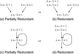
p. Figure 10.3 shows two ways that an expression can be partially redundant. In Figure 10.3a,
a ← b × c occurs on one path leading to the merge point but not on the other. To make the second computation redundant,
lcm inserts an evaluation of
a ← b × c on the other path as shown in Figure 10.3b. In Figure 10.3c,
a ← b × c is redundant along the loop's back edge but not along the edge entering the loop. Inserting an evaluation of
a ← b × c before the loop makes the occurrence inside the loop redundant, as shown in Figure 10.3d. By making the loop-invariant computation redundant and eliminating it,
lcm moves it out of the loop, an optimization called
loopinvariant code motion when performed by itself.
In this context,
earliest means the position in the
cfg closest to the entry node.
The fundamental ideas that underlie
lcm were introduced in Section 9.2.4.
lcm computes both available expressions and anticipable expressions. Next,
lcm uses the results of these analyses to annotate each
cfg edge
 with a set
Earliest(
i,
j) that contains the expressions for which this edge is the
earliest legal placement.
lcm then solves a third data-flow problem to find
later placements, that is, situations where evaluating an expression after its earliest placement has the same effect. Later placements are desirable because they can shorten the lifetimes of values defined by the inserted evaluations. Finally,
lcm computes its final products, two sets
Insert and
Delete, that guide its code-rewriting step.
with a set
Earliest(
i,
j) that contains the expressions for which this edge is the
earliest legal placement.
lcm then solves a third data-flow problem to find
later placements, that is, situations where evaluating an expression after its earliest placement has the same effect. Later placements are desirable because they can shorten the lifetimes of values defined by the inserted evaluations. Finally,
lcm computes its final products, two sets
Insert and
Delete, that guide its code-rewriting step.
Code Shape
lcm relies on several implicit assumptions about the shape of the code. Textually identical expressions always define the same name. Thus, each instance of
r
i + r
j always targets the same
r
k. Thus, the algorithm can use
r
k as a proxy for
r
i + r
j. This naming scheme simplifies the rewriting step; the optimizer can simply replace a redundant evaluation of
r
i + r
j with a copy from
r
k, rather create a new temporary name and insert copies into that name after each prior evaluation.
Notice that these rules are consistent with the register-naming rules described in Section 5.4.2.
lcm moves expression evaluations, not assignments. The naming discipline requires a second rule for program variables because they receive the values of different expressions. Thus, program variables are set by register-to-register copy operations. A simple way to divide the name space between variables and expressions is to require that variables have lower subscripts than any expression, and that in any operation other than a copy, the defined register's subscript must be larger than the subscripts of the operation's arguments. Thus, in
r
i + r
j ⇒ r
k, i < k and
j < k. The example in Figure 10.4 has this property.
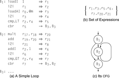
These naming rules allow the compiler to easily separate variables from expressions, shrinking the domain of the sets manipulated in the data-flow equations. In Figure 10.4, the variables are
r
2, r
4, and
r
8, each of which is defined by a copy operation. All the other names
r
1, r
3, r
5, r
6, r
7, r
20, and
r
21, represent expressions. The following table shows the local information for the blocks in the example:
| B 1 | B 2 | B 3 | |
|---|---|---|---|
| DE Expr | {r 1, r 3, r 5} | {r 7, r 20, r 21} | ∅ |
| UE Expr | {r 1, r 3} | {r 6, r 20, r 21} | ∅ |
| E xprK ill | {r 5,r 6,r 7} | {r 5,r 6,r 7} | ∅ |
DE
Expr(
b) is the set of downward-exposed expressions in block
b, UE
Expr(
b) is the set of upward-exposed expressions in
b, and E
xprK
ill(
b) is the set of expressions killed by some operation in
b. We will assume, for simplicity, that the sets for
B3 are all empty.
Available Expressions
The first step in
lcm computes available expressions, in a manner similar to that defined in Section 9.2.4.
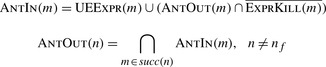
lcm needs availability at the end of the block, so it computes A
vailO
ut rather than A
vailI
n. An expression
e is available on exit from block
b if, along every path from
n0 to
b,
e has been evaluated and none of its arguments has been subsequently defined.
lcm computes A
vailO
ut as follows:
For the example in Figure 10.4, this process produces the following sets:
| B 1 | B 2 | B 3 | |
|---|---|---|---|
| A vailO ut | {r 1, r 3, r 5} | {r 1, r 3, r 7, r 20, r 21} | … |
lcm uses the A
vailO
ut sets to help determine possible placements for an expression in the
cfg. If an expression
e ∈ A
vailO
ut(
b), the compiler could place an evaluation of
e at the end of block
b and obtain the result produced by its most recent evaluation on any control-flow path from
n0 to
b. If
e ∉ A
vailO
ut(
b), then one of
e's constituent subexpressions has been modified since
e's most recent evaluation and an evaluation at the end of block
b would possibly produce a different value. In this light, A
vailO
ut() sets tell the compiler how far forward in the
cfg it can move the evaluation of
e, ignoring any uses of
e.
Anticipable Expressions
To capture information for backward motion of expressions,
lcm computes anticipability. Recall, from Section 9.2.4, that an expression is anticipable at point
p if and only if it is computed on every path that leaves
p and produces the same value at each of those computations. Because
lcm needs information about the anticipable expressions at both the start and the end of each block, we have refactored the equation to introduce a set A
ntI
n(
n) which holds the set of anticipable expressions for the entrance of the block corresponding to node
n in the
cfg.
lcm initializes the A
ntO
ut sets as follows:
Next, it iteratively computes A
ntI
n and A
ntO
ut sets for each block until the process reaches a fixed point.
 |
For the example, this process produces the following sets:
| B 1 | B 2 | B 3 | |
|---|---|---|---|
| A ntI n | {r 1, r 3} | {r 20, r 21} | ∅ |
| A ntO ut | ∅ | ∅ | ∅ |
A
ntO
ut provides information about the safety of hoisting an evaluation to either the start or the end of the current block. If
x ∈ A
ntO
ut(
b), then the compiler can place an evaluation of
x at the end of
b, with two guarantees. First, the evaluation at the end of
b will produce the same value as the next evaluation of
x along any execution path in the procedure. Second, along any execution path leading out of
b, the program will evaluate
x before redefining any of its arguments.
Earliest Placement
Given solutions to availability and anticipability, the compiler can determine, for each expression, the earliest point in the program at which it can evaluate the expression. To simplify the equations,
lcm assumes that it will place the evaluation on a
cfg edge rather than at the start or end of a specific block. Computing an edge placement lets the compiler defer the decision to place the evaluation at the end of the edge's source, at the start of its sink, or in a new block in the middle of the edge. (See the discussion of critical edges in Section 9.3.5.)
For a
cfg edge
 , an expression
e is in
Earliest(
i,
j) if and only if the compiler can legally move
e to
, an expression
e is in
Earliest(
i,
j) if and only if the compiler can legally move
e to
 , and cannot move it to any earlier edge in the
cfg. The
Earliest equation encodes this condition as the intersection of three terms:
, and cannot move it to any earlier edge in the
cfg. The
Earliest equation encodes this condition as the intersection of three terms:
These terms define an earliest placement for
e as follows:
1.
e ∈ A
ntI
n(
j) means that the compiler can safely move
e to the head of
j. The anticipability equations ensure that
e will produce the same value as its next evaluation on any path leaving
j and that each of those paths evaluates
e.
2.
e ∉ A
vailO
ut(
i) shows that no prior computation of
e is available on exit from
i. Were
e ∈ A
vailO
ut(
i), inserting
e on
 would be redundant.
3. The third condition encodes two cases. If
e ∈ E
xprK
ill(
i), the compiler cannot move
e through block
i because of a definition in
i. If
e ∉ A
ntO
ut(
i), the compiler cannot move
e into
i because
e ∉ A
ntI
n(
k) for some edge
 . If either is true, then
e can move no further than
. If either is true, then
e can move no further than
 .
.
The
cfg's entry node,
n0 presents a special case.
lcm cannot move an expression earlier than
n0, so it can ignore the third term in the equation for
Earliest(
n0,
k), for any
k. The
Earliest sets for the continuing example are as follows:
| Earliest | {r 20, r 21} | ∅ | ∅ | ∅ |
Later Placement
The final data-flow problem in
lcm determines when an earliest placement can be deferred to a later point in the
cfg while achieving the same effect.
Later analysis is formulated as a forward data-flow problem on the
cfg with a set L
aterI
n(
n) associated with each node and another set
Later(
i,
j) associated with each edge
 .
lcm initializes the L
aterI
n sets as follows:
.
lcm initializes the L
aterI
n sets as follows:
Next, it iteratively computes L
aterI
n and
Later sets for each block. The computation halts when it reaches a fixed point.
 |
As with availability and anticipability, these equations have a unique fixed point solution.
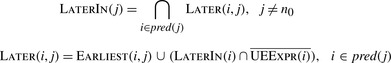
An expression
e ∈ L
aterI
n(
k) if and only if every path that reaches
k includes an edge
 such that
e ∈
Earliest(
p,
q), and the path from
q to
k neither redefines
e's operands nor contains an evaluation of
e that an earlier placement of
e would anticipate. The
Earliest term in the equation for
Later ensures that
Later(
i,
j) includes
Earliest(
i,
j). The rest of that equation puts
e into
Later(
i,
j) if
e can be moved forward from
i, (
e ∈ L
aterI
n(
i)) and a placement at the entry to
i does not anticipate a use in
i, (
e ∉ UE
Expr(
i)).
such that
e ∈
Earliest(
p,
q), and the path from
q to
k neither redefines
e's operands nor contains an evaluation of
e that an earlier placement of
e would anticipate. The
Earliest term in the equation for
Later ensures that
Later(
i,
j) includes
Earliest(
i,
j). The rest of that equation puts
e into
Later(
i,
j) if
e can be moved forward from
i, (
e ∈ L
aterI
n(
i)) and a placement at the entry to
i does not anticipate a use in
i, (
e ∉ UE
Expr(
i)).
Given
Later and L
aterI
n sets,
e ∈ L
aterI
n(
i) implies that the compiler can move the evaluation of
e forward through
i without losing any benefit—that is, there is no evaluation of
e in
i that an earlier evaluation would anticipate, and
e ∈
Later(
i,
j) implies that the compiler can move an evaluation of
e in
i into
j.
For the ongoing example, these equations produce the following sets:
| B 1 | B 2 | B 3 | |
|---|---|---|---|
| L aterI n | ∅ | ∅ | ∅ |
| Later | {r 20, r 21} | ∅ | ∅ | ∅ |
Rewriting the Code
The final step in performing
lcm is to rewrite the code so that it capitalizes on the knowledge derived from the data-flow computations. To drive the rewriting process,
lcm computes two additional sets,
Insert and
Delete.
If
i has only one successor,
lcm can insert the computations at the end of
i. If
j has only one predecessor, it can insert the computations at the entry of
j. If neither condition applies, the edge
 is a critical edge and the compiler should split it by inserting a block in the middle of the edge to evaluate the expressions in
Insert(
i,
j).
is a critical edge and the compiler should split it by inserting a block in the middle of the edge to evaluate the expressions in
Insert(
i,
j).
The
Delete set specifies, for a block, which computations
lcm should delete from the block.
Delete(
n0) is empty, of course, since no block precedes
n0. If
e ∈
Delete(
i), then the first computation of
e in
i is redundant after all the insertions have been made. Any subsequent evaluation of
e in
i that has upward-exposed uses—that is, the operands are not defined between the start of
i and the evaluation—can also be deleted. Because all evaluations of
e define the same name, the compiler need not rewrite subsequent references to the deleted evaluation. Those references will simply refer to earlier evaluations of
e that
lcm has proven to produce the same result.
For our example, the
Insert and
Delete sets are simple.
| Insert | {r 20, r 21} | ∅ | ∅ | ∅ |
| B 1 | B 2 | B 3 | |
|---|---|---|---|
| Delete | ∅ | {r 20, r 21} | ∅ |
The compiler interprets the
Insert and
Delete sets and rewrites the code as shown in Figure 10.5.
lcm deletes the expressions that define
r
20 and
r
21 from
B2 and inserts them on the edge from
B1 to
B2.
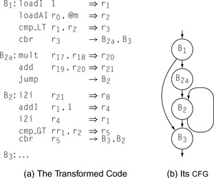
Since
B1 has two successors and
B2 has two predecessors,
 is a critical edge. Thus,
lcm splits the edge, creating a new block
B2a to hold the inserted computations of
r
20 and
r
21. Splitting
is a critical edge. Thus,
lcm splits the edge, creating a new block
B2a to hold the inserted computations of
r
20 and
r
21. Splitting
 adds an extra
jump to the code. Subsequent work in code generation will almost certainly implement the
jump in
B2a as a fall through, eliminating any cost associated with it.
adds an extra
jump to the code. Subsequent work in code generation will almost certainly implement the
jump in
B2a as a fall through, eliminating any cost associated with it.
Coalescing
A pass that determines when a register to register copy can be safely eliminated and the source and destination names combined.
Notice that
lcm leaves the copy defining
r
8 in
B2.
lcm moves expressions, not assignments. (Recall that
r
8 is a variable, not an expression.) If the copy is unnecessary, subsequent copy coalescing, either in the register allocator or as a standalone pass, should discover that fact and eliminate the copy operation.
10.3.2. Code Hoisting
Code motion techniques can also be used to reduce the size of the compiled code. A transformation called
code hoisting provides one direct way of accomplishing this goal. It uses the results of anticipability analysis in a particularly simple way.
If an expression
e ∈ A
ntO
ut(b), for some block
b, that means that
e is evaluated along every path that leaves
b and that evaluating
e at the end of
b would make the first evaluation along each path redundant. (The equations for A
ntO
ut ensure that none of
e's operands is redefined between the end of
b and the next evaluation of
e along each path leaving
b.) To reduce code size, the compiler can insert an evaluation of
e at the end of
b and replace the first occurrence of
e on each path leaving
b with a reference to the previously computed value. The effect of this transformation is to replace multiple copies of the evaluation of
e with a single copy, reducing the overall number of operations in the compiled code.
To replace those expressions directly, the compiler would need to locate them. It could insert
e, then solve another data-flow problem, proving that the path from
b to some evaluation of
e is clear of definitions for
e's operands. Alternatively, it could traverse each of the paths leaving
b to find the first block where
e is defined—by looking in the block's UE
Expr set. Each of these approaches seems complicated.
A simpler approach has the compiler visit each block
b and insert an evaluation of
e at the end of
b, for every expression
e ∈ A
ntO
ut(
b). If the compiler uses a uniform discipline for naming, as suggested in the discussion of
lcm, then each evaluation will define the appropriate name. Subsequent application of
lcm or superlocal value numbering will then remove the newly redundant expressions.
Section Review
Compilers perform code motion for two primary reasons. Moving an operation to a point where it executes fewer times than it would in its original position should reduce execution time. Moving an operation to a point where one instance can cover multiple paths in the
cfg should reduce code size. This section presented an example of each.
lcm is a classic example of a data-flow driven global optimization. It identifies redundant and partially redundant expressions, computes the best place for those expressions, and moves them. By definition, a loop-invariant expression is either redundant or partially redundant;
lcm moves a large class of loop invariant expressions out of loops. Hoisting takes a much simpler approach; it finds operations that are redundant on every path leaving some point
p and replaces all the redundant occurrences with a single instance at
p. Thus, hoisting is usually performed to reduce code size.
The common implementation of sinking is called
cross jumping.
Review Questions
1. Hoisting discovers the situation when some expression
e exists along each path that leaves point
p and each of those occurrences can be replaced safely with an evaluation of
e at
p. Formulate the symmetric and equivalent optimization,
code sinking, that discovers when multiple expression evaluations can safely be moved forward in the code—from points that precede
p to
p.
2. Consider what would happen if you apply your code-sinking transformation during the linker, when all the code for the entire application is present. What effect might it have on procedure linkage code?
10.4. Specialization
In most compilers, the shape of the
ir program is determined by the front end, before any detailed analysis of the code. Of necessity, this produces general code that works in any context that the running program might encounter. With analysis, however, the compiler can often learn enough to narrow the contexts in which the code must operate. This creates the opportunity for the compiler to specialize the sequence of operations in ways that capitalize on its knowledge of the context in which the code will execute.
Major techniques that perform specialization appear in other sections of this book. Constant propagation, described in Sections 9.3.6 and 10.8, analyzes a procedure to discover values that always have the same value; it then folds those values directly into the computation. Interprocedural constant propagation, introduced in Section 9.4.2, applies the same ideas at the whole-program scope. Operator strength reduction, presented in Section 10.4, replaces inductive sequences of expensive computations with equivalent sequences of faster operations. Peephole optimization, covered in Section 11.5, uses pattern matching over short instruction sequences to find local improvement. Value numbering, explained in Section 8.4.1 and Section 8.5.1, systematically simplifies the
ir form of the code by applying algebraic identities and local constant folding. Each of these techniques implements a form of specialization.
Optimizing compilers rely on these general techniques to improve code. In addition, most optimizing compilers contain specialization techniques that specifically target properties of the source languages or applications that the compiler writer expects to encounter. The rest of this section presents three such techniques that target specific inefficiencies at procedure calls: tail-call optimization, leaf-call optimization, and parameter promotion.
10.4.1. Tail-Call Optimization
When the last action that a procedure takes is a call, we refer to that call as a tail call. The compiler can specialize tail calls to their contexts in ways that eliminate much of the overhead from the procedure linkage. To understand how the opportunity for improvement arises, consider what happens when
o calls
p and
p calls
q. When
q returns, it executes its epilogue sequence and jumps back to
p's postreturn sequence. Execution continues in
p until
p returns, at which point
p executes its epilogue sequence and jumps to
o's postreturn sequence.
If the call from
p to
q is a tail call, then no useful computation occurs between the postreturn sequence and the epilogue sequence in
p. Thus, any code that preserves and restores
p's state, beyond what is needed for the return from
p to
o, is useless. A standard linkage, as described in Section 6.5, spends much of its effort to preserve state that is useless in the context of a tail call.
At the call from
p to
q, the minimal precall sequence must evaluate the actual parameters at the call from
p to
q and adjust the access links or the display if necessary. It need not preserve any caller-saves registers, because they cannot be live. It need not allocate a new
ar, because
q can use
p's
ar. It must leave intact the context created for a return to
o, namely the return address and caller's
arp that
o passed to
p and any callee-saves registers that p preserved by writing them into the
ar. (That context will cause the epilogue code for
q to return control directly to
o.) Finally, the precall sequence must jump to a tailored prologue sequence for
q.
In this scheme,
q must execute a custom prologue sequence to match the minimal precall sequence in
p. It only saves those parts of
p's state that allow a return to
o. The precall sequence does not preserve callee-saves registers, for two reasons. First, the values from
p in those registers are no longer live. Second, the values that
p left in the
ar's register-save area are needed for the return to
o. Thus, the prologue sequence in
q should initialize local variables and values that
q needs; it should then branch into the code for
q.
With these changes to the precall sequence in
p and the prologue sequence in
q, the tail call avoids preserving and restoring
p's state and eliminates much of the overhead of the call. Of course, once the precall sequence in
p has been tailored in this way, the postreturn and epilogue sequences are unreachable. Standard techniques such as
Dead and
Clean will not discover that fact, because they assume that the interprocedural jumps to their labels are executable. As the optimizer tailors the call, it can eliminate these dead sequences.
With a little care, the optimizer can arrange for the operations in the tailored prologue for
q to appear as the last operations in its more general prologue. In this scheme, the tail call from
p to
q simply jumps to a point farther into the prologue sequence than would a normal call from some other routine.
If the tail call is a self-recursive call—that is,
p and
q are the same procedure—then tail-call optimization can produce particularly efficient code. In a tail recursion, the entire precall sequence devolves to argument evaluation and a branch back to the top of the routine. An eventual return out of the recursion requires one branch, rather than one branch per recursive invocation. The resulting code rivals a traditional loop for efficiency.
10.4.2. Leaf-Call Optimization
Some of the overhead involved in a procedure call arises from the need to prepare for calls that the callee might make. A procedure that makes no calls, called a leaf procedure, creates opportunities for specialization. The compiler can easily recognize the opportunity; the procedure calls no other procedures.
The other reason to store the return address is to allow a debugger or a performance monitor to unwind the call stack. When such tools are in use, the compiler should leave the save operation intact.
During translation of a leaf procedure, the compiler can avoid inserting operations whose sole purpose is to set up for subsequent calls. For example, the procedure prologue code may save the return address from a register into a slot in the
ar. That action is unnecessary unless the procedure itself makes another call. If the register that holds the return address is needed for some other purpose, the register allocator can spill the value. Similarly, if the implementation uses a display to provide addressability for nonlocal variables, as described in Section 6.4.3, it can avoid the display update in the prologue sequence.
The register allocator should try to use caller-saves registers before callee-saves registers in a leaf procedure. To the extent that it can leave callee-saves registers untouched, it can avoid the save and restore code for them in the prologue and epilogue. In small leaf procedures, the compiler may be able to avoid all use of callee-saves registers. If the compiler has access to both the caller and the callee, it can do better; for leaf procedures that need fewer registers than the caller-save set includes, it can avoid some of the register saves and restores in the caller as well.
In addition, the compiler can avoid the runtime overhead of activation-record allocation for leaf procedures. In an implementation that heap allocates
ars, that cost can be significant. In an application with a single thread of control, the compiler can allocate statically the
ar of any leaf procedure. A more aggressive compiler might allocate one static
ar that is large enough to work for any leaf procedure and have all the leaf procedures share that
ar.
If the compiler has access to both the leaf procedure and its callers, it can allocate space for the leaf procedure's
ar in each of its callers’
ars. This scheme amortizes the cost of
ar allocation over at least two calls—the invocation of the caller and the call to the leaf procedure. If the caller invokes the leaf procedure multiple times, the savings are multiplied.
10.4.3. Parameter Promotion
Ambiguous memory references prevent the compiler from keeping values in registers. Sometimes, the compiler can prove that an ambiguous value has just one corresponding memory location through detailed analysis of pointer values or array subscript values, or special case analysis. In these cases, it can rewrite the code to move that value into a scalar local variable, where the register allocator can keep it in a register. This kind of transformation is often called
promotion. The analysis to promote array references or pointer-based references is beyond the scope of this book. However, a simpler case can illustrate these transformations equally well.
Promotion
A category of transformations that move an ambiguous value into a local scalar name to expose it to register allocation
Consider the code generated for an ambiguous call-by-reference parameter. Such parameters can arise in many ways. The code might pass the same actual parameter in two distinct parameter slots, or it might pass a global variable as an actual parameter. Unless the compiler performs interprocedural analysis to rule out those possibilities, it must treat all reference parameters as potentially ambiguous. Thus, every use of the parameter requires a load and every definition requires a store.
If the compiler can prove that the actual parameter must be unambiguous in the callee, it can promote the parameter's value into a local scalar value, which allows the callee to keep it in a register. If the actual parameter is not modified by the callee, the promoted parameter can be passed by value. If the callee modifies the actual parameter and the result is live in the caller, then the compiler must use value-result semantics to pass the promoted parameter (see Section 6.4.1).
To apply this transformation to a procedure
p, the optimizer must identify all of the call sites that can invoke
p. It can either prove that the transformation applies at all of those call sites or it can clone
p to create a copy that handles the promoted values (see Section 10.6.2). Parameter promotion is most attractive in a language that uses call-by-reference binding.
Section Review
Specialization includes many effective techniques to tailor general-purpose computations to their detailed contexts. Other chapters and sections present powerful global and regional specialization techniques, such as constant propagation, peephole optimization, and operator strength reduction.
This section focused on optimizations that the compiler can apply to the code entailed in a procedure call. Tail-call optimization is a valuable tool that converts tail recursion to a form that rivals conventional iteration for efficiency; it applies to nonrecursive tail calls as well. Leaf procedures offer special opportunities for improvement because the callee can omit major portions of the standard linkage sequence. Parameter promotion is one example of a class of important transformations that remove inefficiencies related to ambiguous references.
Review Questions
1. Many compilers include a simple form of strength reduction, in which individual operations that have one constant-valued operand are replaced by more efficient, less general operations. The classic example is replacing an integer multiply of a positive number by a series of shifts and adds. How might you fold that transformation into local value numbering?
2. Inline substitution might be an alternative to the procedure-call optimizations in this section. How might you apply inline substitution in each case? How might the compiler choose the more profitable alternative?
10.5. Redundancy Elimination
A computation
x +
y is redundant at some point
p in the code if, along every path that reaches
p,
x +
y has already been evaluated and
x and
y have not been modified since the evaluation. Redundant computations typically arise as artifacts of translation or optimization.
We have already presented three effective techniques for redundancy elimination: local value numbering
lvn in Section 8.4.1, superlocal value numbering
svn in Section 8.5.1 and lazy code motion (
lcm) in Section 10.3.1. These algorithms cover the span from simple and fast
lvn to complex and comprehensive (
lcm). While all three methods differ in the scope that they cover, the primary distinction between them lies in the method that they use to establish that two values are identical. The next section explores this issue in detail. The second section presents one more version of value numbering, a dominator-based technique.
10.5.1. Value Identity versus Name Identity
lvn introduced a simple mechanism to prove that two expressions had the same value.
lvn relies on two principles. It assigns each value a unique identifying number—its value number. It assumes that two expressions produce the same value if they have the same operator and their operands have the same value numbers. These simple rules allow
lvn to find a broad class of redundant operations—any operation that produces a pre-existing value number is redundant.
With these rules,
lvn can prove that 2 +
a has the same value as
a + 2 or as 2 + b when
a and
b have the same value number. It cannot prove that
a +
a and 2 ×
a have the same value because they have different operators. Similarly, it cannot prove the
a + 0 and
a have the same value. Thus, we extend
lvn with algebraic identities that can handle the well-defined cases not covered by the original rule. The table in Figure 8.3 on page 424 shows the range of identities that
lvn can handle.
By contrast,
lcm relies on names to prove that two values have the same number. If
lcm sees
a +
b and
a +
c, it assumes that they have different values because
b and
c have different names. It has relies on a lexical comparison—name identity. The underlying data-flow analyses cannot directly accommodate the notion of value identity; data-flow problems operate a predefined name space and propagate facts about those names over the
cfg. The kind of ad hoc comparisons used in
lvn do not fit into the data-flow framework.
As described in Section 10.6.4, one way to improve the effectiveness of
lcm is to encode value identity into the name space of the code before applying
lcm.
lcm recognizes redundancies that neither
lvn nor
svn can find. In particular, it finds redundancies that lie on paths through join points in the
cfg, including those that flow along loop-closing branches, and it finds partial redundancies. On the other hand, both
lvn and
svn find value-based redundancies and simplifications that
lcm cannot find. Thus, encoding value identity into the name space allows the compiler to take advantage of the strengths of both approaches.
10.5.2. Dominator-Based Value Numbering
 |
Chapter 8 presented both local value numbering
lvn and its extension to extended basic blocks (
Ebbs), called superlocal value numbering
svn. While
svn discovers more redundancies than
lvn, it still misses some opportunities because it is limited to
Ebbs. Recall that the
svn algorithm propagates information along each path through an
Ebb. For example, in the
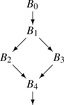
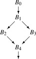
cfg fragment shown in the margin,
svn will process the paths (
B0,
B1,
B2) and (
B0,
B1,
B3). Thus, it optimizes both
B2 and
B3 in the context of the prefix path (
B0,
B1). Because
B4 forms its own degenerate
Ebb,
svn optimizes
B4 without prior context.
From an algorithmic point of view,
svn begins each block with a table that includes the results of all predecessors on its
Ebb path. Block
B4 has no predecessors, so it begins with no prior context. To improve on that situation, we must answer the question: on what state could
B4 rely?
B4 cannot rely on values computed in either
B2 or
B3, since neither lies on every path that reaches
B4. By contrast,
B4 can rely on values computed in
B0 and
B1, since they occur on every path that reaches
B4. Thus, we might extend value numbering for
B4 with information about computations in
B0 and
B1. We must, however, account for the impact of assignments in the intervening blocks,
B2 or
B3.
Consider an expression,
x +
y, that occurs at the end of
B1 and again at the start of
B4. If neither
B2 or
B3 redefines
x or
y, then the evaluation of
x +
y in
B4 is redundant and the optimizer can reuse the value computed in
B1. On the other hand, if either of those blocks redefines
x or
y, then the evaluation of
x +
y in
B4 computes a distinct value from the evaluation in
B1 and the evaluation is not redundant.
Fortunately, the
ssa name space encodes precisely this distinction. In
ssa, a name that is used in some block
B
i can only enter
B
i in one of two ways. Either the name is defined by a
ϕ-function at the top of
B
i, or it is defined in some block that dominates
B
i. Thus, an assignment to
x in either
B2 or
B3 creates a new name for
x and forces the insertion of a
ϕ-function for
x at the head of
B4. That
ϕ-function creates a new
ssa name for
x and the renaming process changes the
ssa name used in the subsequent computation of
x +
y. Thus,
ssa form encodes the presence or absence of an intervening assignment in
B2 or
B3 directly into the names used in the expression. Our algorithm can rely on
ssa names to avoid this problem.
The other major question that we must answer before we can extend
svn to larger regions is, given a block such as
B4, how do we locate the most recent predecessor with information that the algorithm can use? Dominance information, discussed at length in Section 9.2.1 and Section 9.3.2, captures precisely this effect.
Dom(
B4) = {
B0,
B1,
B4}.
B4's immediate dominator, defined as the node in (
Dom(
B4) −
B4) that is closest to
B4, is
B1, the last node that occurs on all path from the entry node
B0 to
B4.
The dominator-based value numbering technique
dvnt builds on the ideas behind
svn. It uses a scoped hash table to hold value numbers.
dvnt opens a new scope for each block and discards that scope when they are no longer needed.
dvnt actually uses
ssa names as value numbers; thus the value number for an expression
ai ×
bj is the
ssa name defined in the first evaluation of
ai ×
bj. (That is, if the first evaluation occurs in
tk ←
ai ×
bj, then the value number for
ai ×
bj is
tk.)
Figure 10.6 shows the algorithm. It takes the form of a recursive procedure that the optimizer invokes on a procedure's entry block. It follows both the
cfg for the procedure, represented by the dominator tree, and the flow of values in the
ssa form. For each block
B,
dvnt takes three steps: it processes the
ϕ-functions in
B, if any exist, it value numbers the assignments, and it propagates information into
B's successors and recurs on
B's children in the dominator tree.
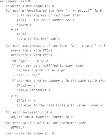
Process the ϕ-Functions in B
dvnt must assign each
ϕ-function
p a value number. If
p is meaningless—that is, all its arguments have the same value number—
dvnt sets its value number to the value number for one of its arguments and deletes
p. If
p is redundant—that is, it produces the same value number as another
ϕ-function in
B—
dvnt assigns
p the same value number as the
ϕ-function that it duplicates.
dvnt then deletes
p.
Otherwise, the
ϕ-function computes a new value. Two cases arise. The arguments to
p have value numbers, but the specific combination of arguments have not been seen before in this block, or one or more of
p's arguments has no value number. The latter case can arise from a back edge in the
cfg.
Process the Assignments in B
Recall, from the
ssa construction, that uninitialized names are not allowed.
dvnt iterates over the assignments in
B and processes them in a manner analogous to
lvn and
svn. One subtlety arises from the use of
ssa names as value numbers. When the algorithm encounters a statement
x ←
y op z, it can simply replace
y with
VN[y] because the name in
VN[y] holds the same value as
y.
Propagate Information to B's Successors
Once
dvnt has processed all the
ϕ-functions and assignments in
B, it visits each of
B's
cfg successors
s and updates
ϕ function arguments that correspond to values flowing across the edge (
b,
s). It records the current value number for the argument in the
ϕ-function by overwriting the argument's
ssa name. (Notice the similarity between this step and the corresponding step in the renaming phase of the
ssa construction.) Next, the algorithm recurs on
B's children in the dominator tree. Finally, it deallocates the hash table scope that it used for
B.
This recursion scheme causes
dvnt to follow a preorder walk on the dominator tree, which ensures that the appropriate tables have been constructed before it visits a block. This order can produce a counterintuitive traversal; for the
cfg in the margin, the algorithm could visit
B4 before either
B2 or
B3. Since the only facts that the algorithm can use in
B4 are those discovered processing
B0 and
B1, the relative ordering of
B2,
B3, and
B4 is not only unspecified, it is also irrelevant.
 |
Section Review
Redundancy elimination operates on the assumption that it is faster to reuse a value than to recompute it. Building on that assumption, these methods identify as many redundant computations as possible and eliminate duplicate computation. The two primary notions of equivalence used by these transformations are value identity and name identity. These different tests for identity produce different results.
Both value numbering and
lcm eliminate redundant computation.
lcm eliminates redundant and partially redundant expression evaluation; it does not eliminate assignments. Value numbering does not recognize partial redundancies, but it can eliminate assignments. Some compilers use a value-based technique, such as
dvnt, to discover redundancy and then encode that information into the name space for a name-based transformation such as
lcm. In practice, that approach combines the strength of both ideas.
Review Questions
1. The
dvnt algorithm resembles the renaming phase of the
ssa construction algorithm. Can you reformulate the renaming phase so that it performs value numbering as it renames values? What impact would this change have on the size of the
ssa form for a procedure?
2. The
dvnt algorithm does not propagate a value along a loop-closing edge—a back edge in the call graph.
lcm will propagate information along such edges. Write several examples of redundant expressions that a true “global” technique such as
lcm can find that
dvnt cannot.
10.6. Enabling Other Transformations
Often, an optimizer includes passes whose primary purpose is to create or expose opportunities for other transformations. In some cases, a transformation changes the shape of the code to make it more amenable to optimization. In other cases, the transformation creates a point in the code where specific conditions hold that make another transformation safe. By directly creating the necessary code shape, these enabling transformations reduce the sensitivity of the optimizer to the shape of the input code.
Several enabling transformations are described in other parts of the book. Both loop unrolling (Section 8.5.2) and inline substitution (Section 8.7.1) obtain most of their benefits by creating context for other optimization. (In each case, the transformation does eliminate some overhead, but the larger effect comes from subsequent application of other optimizations.) The tree-height balancing algorithm (Section 8.4.2) does not eliminate any operations, but it creates a code shape that can produce better results from instruction scheduling. This section presents four enabling transformations:
superblock cloning,
procedure cloning,
loop unswitching, and
renaming.
10.6.1. Superblock Cloning
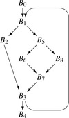 |
Often, the optimizer's ability to transform the code is limited by path-specific information in the code. Imagine using
svn on the
cfg shown in the margin. The fact that blocks
B3 and
B7 have multiple predecessors may limit the optimizer's ability to improve code in those blocks. If, for example, block
B6 assigned
x the value 7 and block
B8 assigned
x the value 13, a use of
x in
B7 would appear to receive the value ⊥, even though the value is known and predictable along each path leading to
B7.
In such circumstances, the compiler can clone blocks to create code that is better suited for the transformation. In this case, it might create two copies of
B7, say
B7
a and
B7
b, and redirect the incoming edges as
 and
and
 . With this change, the optimizer could propagate the value 7 for
x into
B7
a and the value 13 for
x into
B7
b.
. With this change, the optimizer could propagate the value 7 for
x into
B7
a and the value 13 for
x into
B7
b.
As an additional benefit, since
B7
a and
B7
b both have unique predecessors, the compiler can actually merge the blocks to create a single block from
B6 and
B7
a and another from
B8 and
B7
b. This transformation eliminates the block-ending jump in
B6 and
B8 and, potentially, allows for further improvement in optimization and in instruction scheduling.
Backward Branch
a
cfg edge whose destination has a lower depth-first number than its source, with respect to some depth-first traversal of the
cfg
An issue in this kind of cloning is, when should the compiler stop cloning? One cloning technique, called
superblock cloning, is widely used to create additional context for instruction scheduling inside loops. In superblock cloning, the optimizer starts with a loop head—the entry to a loop—and clones each path until it reaches a backward branch.
Applying this technique to the example
cfg produces the modified
cfg shown in the margin.
B1 is the loop header. Each of the nodes in the loop body has a unique predecessor. If the compiler applies a superlocal optimization (one based on extended basic blocks), every path that it finds will encompass a single iteration of the loop body. (To find longer paths, the optimizer would need to unroll the loop so that superblock cloning encompassed multiple iterations.)
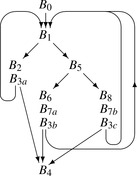 |
Superblock cloning can improve the results of optimization in three principal ways.
1.
It creates longer blocks Longer blocks let local optimization handle more context. In the case of value numbering, the superlocal and dominator versions are as strong as the local version. For some techniques, however, this is not the case. For instruction scheduling, for example, superlocal and dominator versions are weaker than the local method. In that case, cloning, followed by local optimization, can produce better code.
2.
It eliminates branches Combining two blocks eliminates a branch between them. Branches take time to execute. They also disrupt some of the performance-critical mechanisms in the processor, such as instruction fetching and many of the pipelined functions. The net effect of removing branches is to shorten execution time, by eliminating operations and by making hardware mechanisms for predicting behavior more effective.
3.
It creates points where optimization can occur When cloning eliminates a control-flow merge point, it creates new points in the program where the compiler can derive more precise knowledge about the runtime context. The transformed code may present opportunities for specialization and redundancy elimination that exist nowhere in the original code.
Of course, cloning has costs, too. It creates multiple copies of individual operations, which leads to larger code. The larger code may run more quickly because it avoids some end-of-block jumps. It may run more slowly if its size causes additional instruction cache misses. In applications where the user cares more about code space than runtime speed, superblock cloning may be counterproductive.
10.6.2. Procedure Cloning
Inline substitution, described in Section 8.7.1 on page 458, has effects similar to superblock cloning. For a call from
p to
q, it creates a unique copy of
q and merges it with the call site in
p. The same effects that arise with superblock cloning arise with inline substitution, including specialization to a particular context, elimination of some control-flow operations, and increased code size.
In some cases, the compiler can achieve some of the benefits of inline substitution with less code growth by cloning the procedure. The idea is analogous to the block cloning that occurs in superblock cloning. The compiler creates multiple copies of the callee and assigns some of the calls to each instance of the clone.
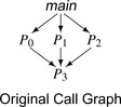 |
Careful assignment of calls to clones can create situations where every call has a similar context for optimization. Consider, for example, the simple call graph shown in the margin. Assume that
P3 is a library routine whose behavior depends strongly on one of its input parameters; for a value of one, the compiler can generate code that provides efficient memory access, while for other values, it produces much larger, slower code. Further, assume that
P0 and
P1 both pass it the value 1, while
P2 passes it the value 17.
 |
Constant propagation across the call graph does not help here because it must compute the parameter as
 . With constant propagation alone, the compiler must still generate the fully general code for
P3. Procedure cloning can create a place where the parameter is always 1;
P3
a in the graph in the margin. The call that inhibits optimization, (
P2,
P3) in the original call graph, is assigned to
P3
b. The compiler can generate optimized code for
P3
a and the general code for
P3
b.
. With constant propagation alone, the compiler must still generate the fully general code for
P3. Procedure cloning can create a place where the parameter is always 1;
P3
a in the graph in the margin. The call that inhibits optimization, (
P2,
P3) in the original call graph, is assigned to
P3
b. The compiler can generate optimized code for
P3
a and the general code for
P3
b.
10.6.3. Loop Unswitching
Loop unswitching hoists loop-invariant control-flow operations out of a loop. If the predicate in an
if-then-else construct is loop invariant, then the compiler can rewrite the loop by pulling the
if-then-else out of the loop and generating a tailored copy of the loop inside each half of the new
if-then-else. Figure 10.7 shows this transformation for a short loop.
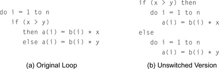
Unswitching is an enabling transformation; it allows the compiler to tailor loop bodies in ways that are otherwise hard to achieve. After unswitching, the remaining loops contain less control flow. They execute fewer branches and other operations to support those branches. This can lead to better scheduling, better register allocation, and faster execution. If the original loop contained loop-invariant code that was inside the
if-then-else, then
lcm could not move it out of the loop. After unswitching,
lcm easily finds and removes such redundancies.
Unswitching also has a simple, direct effect that can improve a program: it moves the branching logic that governs the loop-invariant conditional out of the loop. Moving control flow out of loops is difficult. Techniques based on data-flow analysis, like
lcm, have trouble moving such constructs because the transformation modifies the
cfg on which the analysis relies. Techniques based on value numbering can recognize cases where the predicates controlling
if-then-else constructs are identical, but typically cannot remove the construct from a loop.
10.6.4. Renaming
Most scalar transformations rewrite or reorder the operations in the code. We have seen, at several points in the text, that the choice of names can either obscure or expose opportunities for improvement. For example, in
lvn, converting the names in a block to the
ssa name space exposed some opportunities for reuse that would otherwise be difficult to capture.
For many transformations, careful construction of the “right” name space can expose additional opportunities, either by making more facts visible to analysis or by avoiding some of the side effects that arise from reuse of storage. As an example, consider
lcm. Because it relies on data-flow analysis to identify opportunities, the analysis relies on a notion of lexical identity—redundant operations must have the same operation and their operands must have the same names. Thus,
lcm cannot discover that
x +
x and
2 ·
x have the same value, or that
x +
x and
x +
y have the same value when
x =
y.
To improve the results of
lcm, the compiler can encode value identity into the name space before it applies
lcm. The compiler would use a value-based redundancy technique, such as
dvnt, and then rewrite the name space so that equivalent values share the same name. By encoding value identity into lexical identity, the compiler exposes more redundancy to
lcm and makes it more effective.
In a similar way, names matter to instruction scheduling. In a scheduler, names encode the data dependences that constrain the placement of operations in the scheduled code. When the reuse of a name reflects the actual flow of values, that reuse provides critical information required for correctness. If reuse of a name occurs because a prior pass has compressed the name space, then the reuse may unnecessarily constrain the schedule. For example, the register allocator places distinct values into the same physical register to improve register utilization. If the compiler performs allocation before scheduling, the allocator can introduce apparent constraints on the scheduler that are not required by the original code.
The illusion of a constraint introduced by naming is often called
false sharing.
Renaming is a subtle issue. Individual transformations can benefit from name spaces with different properties. Compiler writers have long recognized that moving and rewriting operations can improve programs. In the same way, they should recognize that renaming can improve optimizer effectiveness. As
ssa has shown, the compiler need not be bound by the name space introduced by the programmer or by the compiler's front end. Renaming is a fertile ground for future work.
Section Review
As we saw in Chapter 7,, the shape of the
ir for a procedure has an effect on the code that the compiler can generate for it. The techniques discussed in this section create opportunities for other optimizations by changing the shape of the code. They use replication, selective rewriting, and renaming to create places in the code that are amenable to improvement by specific transformations.
Cloning, at the block level or the procedure level, achieves its effects by eliminating the deleterious effects that occur at control-flow merge points. As it eliminates edges, in either the
cfg or the call graph, cloning also creates opportunities to merge code. Loop unswitching performs specialized code motion of control structures, but its primary benefit derives from creating simpler loops that do not contain conditional control flow. This latter benefit improves results from transformations that range from
lcm to instruction scheduling. Renaming is a powerful idea with widespread application; the specific case of encoding value identity into lexical identity has proven itself in several well-known compilers.
Review Questions
1. Superblock cloning creates new opportunities for other optimizations. Consider tree-height balancing. How much can superblock cloning help? Can you envision a transformation to follow superblock cloning that would expose more opportunities for tree-height balancing? For
svn, how might the results of using
svn after cloning compare to the results of running
lcm on the same code?
2. Procedure cloning attacks some of the same inefficiencies as inline substitution. Is there a role for both of these transformations in a single compiler? What are the potential benefits and risks of each transformation? How might a compiler chose between them?
The SSA Graph
In some algorithms, viewing the
ssa form of the code as a graph simplifies either the discussion or the implementation. The algorithm for strength reduction interprets the
ssa form of the code as a graph.
In
ssa form, each name has a unique definition, so that a name specifies a particular operation in the code that computed its value. Each use of a name occurs in a specific operation, so the use can be interpreted as a chain from the use to its definition. Thus, a simple lookup table that maps names to the operations that define them creates a chain from each use to the corresponding definition. Mapping a definition to the operations that use it is slightly more complex. However, this map can easily be constructed during the renaming phase of the
ssa construction.
We draw
ssa graphs with edges that run from a use to its corresponding definition. This indicates the relationship implied by the
ssa names. The compiler needs to traverse the edges in both directions. Strength reduction moves, primarily, from uses to definitions. The
sccp algorithm transmits values from definitions to uses. The compiler writer can easily add the data structures needed to allow traversal in both directions.
10.7. Advanced Topics
Most of the examples in this chapter have been chosen to illustrate a specific effect that the compiler can use to speed up the executable code. Sometimes, performing two optimizations together can produce results that cannot be obtained with any combination of applying them separately. The next subsection shows one such example: combining constant propagation with unreachable code elimination. Section 10.7.2 presents a second, more complex example of specialization: operator strength reduction with linear function test replacement. The algorithm that we present,
OSR, is simpler than previous algorithms because it relies on properties of
ssa form. Finally, Section 10.7.3 discusses some of the issues that arise in choosing a specific application order for the optimizer's set of transformations.
10.7.1. Combining Optimizations
Sometimes, reformulating two distinct optimizations in a unified framework and solving them jointly can produce results that cannot be obtained by any combination of the optimizations run separately. As an example, consider the sparse simple constant propagation (
sscp) algorithm described in Section 9.3.6. It assigns a lattice value to the result of each operation in the ssa form of the program. When it halts, it has tagged every definition with a lattice value that is either ⊤, ⊥, or a constant. A definition can have the value ⊤ only if it relies on an uninitialized variable or it occurs in an unreachable block.
sscp assigns a lattice value to the operand used by a conditional branch. If the value is ⊥, then either branch target is reachable. If the value is neither ⊥ nor ⊤, then the operand must have a known value and the compiler can rewrite the branch with a jump to one of its two targets, simplifying the
cfg. Since this removes an edge from the
cfg, it may make the block that was the branch target unreachable. Constant propagation can ignore any effects of an unreachable block.
sscp has no mechanism to take advantage of this knowledge.
We can extend the
sscp algorithm to capitalize on these observations. The resulting algorithm, called
sparse conditional constant propagation (
sccp), appears in Figure 10.8, Figure 10.9 and Figure 10.10.
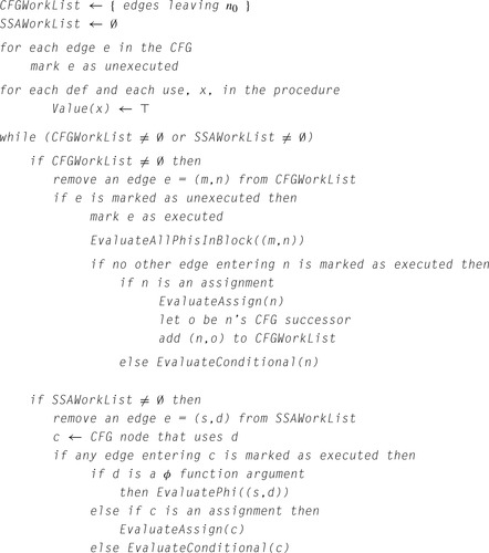
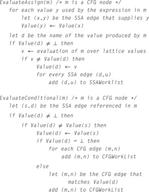
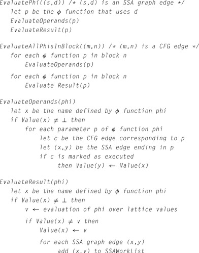
In concept,
sccp operates in a straightforward way. It initializes the data structures. It iterates over two graphs, the
cfg and the
ssa graph. It propagates reachability information on the
cfg and value information on the
ssa graph. It halts when the value information reaches a fixed point; because the constant propagation lattice is so shallow, it halts quickly. Combining these two kinds of information,
sccp can discover both unreachable code and constant values that the compiler simply could not discover with any combination of the
sscp and unreachable code elimination.
To simplify the explanation of
sccp, we assume that each block in the
cfg represents just one statement, plus some optional
ϕ-functions. A
cfg node with a single predecessor holds either an assignment statement or a conditional branch. A
cfg node with multiple predecessors holds a set of
ϕ-functions, followed by an assignment or a conditional branch.
In detail,
sccp is much more complex than either
sscp or unreachable code elimination. Using two graphs introduces additional bookkeeping. Making the flow of values depend on reachability introduces additional work to the algorithm. The result is a powerful but complex algorithm.
The algorithm proceeds as follows. It initializes each
Value field to ⊤ and marks each
cfg edge as “unexecuted.” It initializes two worklists, one for
cfg edges and the other for
ssa graph edges. The
cfg worklist receives the set of edges that leave the procedure's entry node,
n0. The
ssa worklist receives the empty set.
After the initialization phase, the algorithm repeatedly picks an edge from one of the two worklists and processes that edge. For a
cfg edge (
m,
n),
sccp determines if the edge is marked as executed. If (
m,
n) is so marked,
sccp takes no further action for (
m,
n). If (
m,
n) is marked as unexecuted, then
sccp marks it as executed and evaluates all of the
ϕ-functions at the start of block
n. Next,
sccp determines if block
n has been previously entered along another edge. If it has not, then
sccp evaluates the assignment or conditional branch in
n. This processing may add edges to either worklist.
In this discussion, a block is
reachable if and only if some
CFG edge that enters it is marked as executable.
For an
ssa edge, the algorithm first checks if the destination block is reachable. If the block is reachable,
sccp calls one of
EvaluatePhi,
EvaluateAssign, or
EvaluateConditional, based on the kind of operation that uses the
ssa name. When
sccp must evaluate an assignment or a conditional over the lattice of values, it follows the same scheme used in
sscp, discussed in Section 9.3.6 on page 515. Each time the lattice value for a definition changes, all the uses of that name are added to the
ssa worklist.
Because
sccp only propagates values into blocks that it has already proved executable, it avoids processing unreachable blocks. Because each value propagation step is guarded by a test on the executable flag for the entering edge, values from unreachable blocks do not flow out of those blocks. Thus, values from unreachable blocks have no role in setting the lattice values in other blocks.
After the propagation step, a final pass is required to replace operations that have operands with
Value tags other than ⊥. It can specialize many of these operations. It should also rewrite branches that have known outcomes with the appropriate jump operations. Later passes can remove the unreachable code (see Section 10.2). The algorithm cannot rewrite the code until the propagation completes.
Subtleties in Evaluating and Rewriting Operations
Some subtle issues arise in modeling individual operations. For example, if the algorithm encounters a multiply operation with operands ⊤ and ⊥, it might conclude that the operation produces ⊥. Doing so, however, is premature. Subsequent analysis might lower the ⊤ to the constant 0, so that the multiply produces a value of 0. If
sccp uses the rule ⊤ × ⊥ → ⊥, it introduces the potential for nonmonotonic behavior—the multiply's value might follow the sequence ⊤, ⊥, 0, which would increase the running time of
sccp. Equally important, it might incorrectly drive other values to ⊥ and cause
sccp to miss opportunities for improvement.
To address this,
sccp should use three rules for multiplies that involve ⊥, as follows: ⊤ × ⊥ → ⊤,
α × ⊥ → ⊥ for
α ≠ ⊤ and
α ≠ 0, and 0 × ⊥ → 0. This same effect occurs for any operation for which the value of one argument can completely determine the result. Other examples include a shift by more than the word length, a logical
and with zero, and a logical
or with all ones.
Some rewrites have unforeseen consequences. For example, replacing 4 ×
s, for nonnegative
s, with a shift replaces a commutative operation with a noncommutative operation. If the compiler subsequently tries to rearrange expressions using commutativity, this early rewrite forecloses an opportunity. This kind of interaction can have noticeable effects on code quality. To choose when the compiler should convert 4 ×
s into a shift, the compiler writer must consider the order in which optimizations will be applied.
Effectiveness
sccp can find constants that the
sscp algorithm cannot. Similarly, it can discover unreachable code that no combination of the algorithms in Section 10.2 can discover. It derives its power from combining reachability analysis with the propagation of lattice values. It can eliminate some
cfg edges because the lattice values are sufficient to determine which path a branch takes. It can ignore
ssa edges that arise from unreachable operations (by initializing those definitions to ⊤) because those operations will be evaluated if the block becomes marked as reachable. The power of
sccp arises from the interplay between these analyses—constant propagation and reachability.
If reachability did not affect the final lattice values, then the same effects could be achieved by performing constant propagation (and rewriting constant-valued branches as jumps) followed by unreachable-code elimination. If constant propagation played no role in reachability, then the same effects could be achieved by the other order—unreachable-code elimination followed by constant propagation. The power of
sccp to find simplifications beyond those combinations comes precisely from the fact that the two optimizations are interdependent.
10.7.2. Strength Reduction
Operator strength reduction is a transformation that replaces a repeated series of expensive (“strong”) operations with a series of inexpensive (“weak”) operations that compute the same values. The classic example replaces integer multiplications based on a loop index with equivalent additions. This particular case arises routinely from the expansion of array and structure addresses in loops. Figure 10.11a shows the
iloc that might be generated for the following loop:
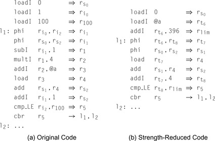
sum ← 0
for i ← 1 to 100
sum ← sum + a(i)
The code is in semipruned
ssa form; the purely local values (
r
2, r
2, r
3, and
r
4) have neither subscripts nor
ϕ-functions. Notice how the reference to
a(i) expands to four operations—the
subI,
multI, and
addI that compute
(i − 1) × 4 − @a and the
load that defines
r
4.
For each iteration, this sequence of operations computes the address of
a(i) from scratch as a function of the loop index variable
i. Consider the sequences of values taken on by
r
i
1, r
1, r
2, and r
3.
r
i
1: {1, 2, 3, …, 100}
r
1: {0, 1, 2, …, 99}
r
2: {0, 4, 8, …, 396}
r
3: {
@a, @a+4,
@a+8, …,
@a+396}
The values in
r
1,
r
2, and
r
3 exist solely to compute the address for the
load operation. If the program computed each value of
r
3 from the preceding one, it could eliminate the operations that define
r
1 and
r
2. Of course,
r
3 would then need an initialization and an update. This would make it a nonlocal name, so it would also need a
ϕ-function at both
l
1 and
l
2.
Figure 10.11b shows the code after strength reduction, linear-function test replacement, and dead-code elimination. It computes those values formerly in
r
3 directly into
r
t
7 and uses
r
t
7 in the
load operation. The end-of-loop test, which used
r
1 in the original code, has been modified to use
r
t
8. This makes the computations of
r
1,
r
2,
r
3,
r
i
0,
r
i
1, and
r
i
2 all dead. They have been removed to produce the final code. Now, the loop contains just five operations, ignoring
ϕ-functions, while the original code contained eight. (In translating from
ssa form back to executable code, the
ϕ-functions become copy operations that the register allocator can usually remove.)
If the
multI operation is more expensive than an
addI, the savings will be larger. Historically, the high cost of multiplication justified strength reduction. However, even if multiplication and addition have equal costs, the strength-reduced form of the loop may be preferred because it creates a better code shape for later transformations and for code generation. In particular, if the target machine has an autoincrement addressing mode, then the
addI operation in the loop can be folded into the memory operation. This option simply does not exist for the original multiply.
The rest of this section presents a simple algorithm for strength reduction, which we call
OSR, followed by a scheme for linear function test replacement that shifts end-of-loop tests away from variables that would otherwise be dead.
OSR operates on the
ssa form of the code, considered as a graph. Figure 10.12 shows the code for our example, alongside its
ssa graph.
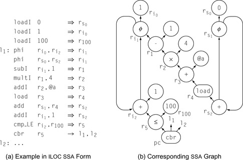
Background
Region Constant
A value that does not vary within a given loop is a
region constant for that loop.
Induction Variable
A value that increases or decreases by a constant amount in each iteration of a loop is an
induction variable.
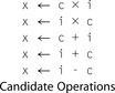 |
Strength reduction looks for contexts in which an operation, such as a multiply, executes inside a loop and its operands are (1) a value that does not vary in that loop, called a
region constant, and (2) a value that varies systematically from iteration to iteration, called an
induction variable. When it finds this situation, it creates a new induction variable that computes the same sequence of values as the original multiplication in a more efficient way. The restrictions on the form of the multiply operation's operands ensure that this new induction variable can be computed using additions, rather than multiplications.
We call an operation that can be reduced in this way a
candidate operation. To simplify the presentation of
OSR, we consider only candidate operations that have one of the five forms shown in the margin, where
c is a region constant and
i is an induction variable. The key to finding and reducing candidate operations is efficient identification of region constants and induction variables. An operation is a candidate if and only if it has one of these forms, including the restrictions on operands.
A region constant can either be a literal constant, such as 10, or a loop-invariant value, that is, one not modified inside the loop. With the code in
ssa form, the compiler can determine if an argument is loop invariant by checking the location of its sole definition—its definition must dominate the entry to the loop that defines the induction variable.
OSR can check both of these conditions in constant time. Performing
lcm and constant propagation before strength reduction may expose more region constants.
Intuitively, an induction variable is a variable whose values in the loop form an arithmetic progression. For the purposes of this algorithm, we can use a much more specific and restricted definition: an induction variable is a strongly connected component (
scc) of the
ssa graph in which each operation that updates its value is one of (1) an induction variable plus a region constant, (2) an induction variable minus a region constant, (3) a
ϕ-function, or (4) a register-to-register copy from another induction variable. While this definition is much less general than conventional definitions, it is sufficient to enable the
OSR algorithm to find and reduce candidate operations. To identify induction variables,
OSR finds
sccs in the
ssa graph and iterates over them to determine if each operation in the
scc is of one of these four types.
Because
OSR defines induction variables in the
ssa graph and region constants relative to a loop in the
cfg, the test to determine if a value is constant relative to the loop containing a specific induction variable is complicated. Consider an operation
o of the form
x ← i × c, where
i is an induction variable. For
o to be a candidate for strength reduction,
c must be a region constant with respect to the outermost loop in which
i varies. To test whether
c has this property,
OSR must relate the
scc for
i in the
ssa graph back to a loop in the
cfg.
OSR finds the
ssa graph node with the lowest reverse postorder number in the
scc defining
i. It considers this node to be the header of the
scc and records that fact in the header field of each node of the
scc. (Any node in the
ssa graph that is not part of an induction variable has its header field set to
null.) In
ssa form, the induction variable's header is the
ϕ-function at the start of the outermost loop in which it varies. In an operation
x ← i × c, where
i is an induction variable,
c is a region constant if the
cfg block that contains its definition dominates the
cfg block that contains
i's header. This condition ensures that
c is invariant in the outermost loop in which
i varies. To perform this test, the
ssa construction must produce a map from each
ssa node to the
cfg block where it originated.
The header field plays a critical role in determining whether or not an operation can be strength reduced. When
OSR encounters an operation
x ← y × z, it can determine if
y is an induction variable by following the
ssa graph edge to
y's definition and inspecting its header field. A
null header field indicates that
y is not an induction variable. If both
y and
z have
null header fields, the operation cannot be strength reduced.
If one of
y or
z has a non-
null header field, then
OSR uses that header field to determine if the other operand is a region constant. Assume
y's header is not
null. To find the
cfg block for the entry to the outermost loop where
y varies,
OSR consults the
ssa-to-
cfg map, indexed by
y's header. If the
cfg block containing
z's definition dominates the
cfg block of
y's header, then
z is a region constant relative to the induction variable
y.
The Algorithm
To perform strength reduction,
OSR must examine each operation and determine if one of its operands is an induction variable and the other is a region constant. If the operation meets these criteria,
OSR can reduce it by creating a new induction variable that computes the needed values and replacing the operation with a register-to-register copy from this new induction variable. (It should avoid creating duplicate induction variables.)
Based on the preceding discussion, we know that
OSR can identify induction variables by finding
sccs in the
ssa graph. It can discover a region constant by examining the value's definition. If the definition results from an immediate operation, or its
cfg block dominates the
cfg block of the induction variable's header, then the value is a region constant. The key is putting these ideas together into an efficient algorithm.
OSR uses Tarjan's strongly connected region finder to drive the entire process. As shown in Figure 10.13,
OSR takes an
ssa graph as its argument and repeatedly applies the strongly connected region finder,
DFS, to it. (This process stops when
DFS has visited every node in
G.)
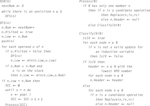
DFS performs a depth-first search of the
ssa graph. It assigns each node a number, corresponding to the order in which it visits the node. It pushes each node onto a stack and labels the node with the lowest depth-first number on a node that can be reached from its children. When it returns from processing the children, if the lowest node reachable from
n has
n's number, then
n is the header of an
scc.
DFS pops nodes off the stack until it reaches
n; all of those nodes are members of the
scc.
DFS removes
sccs from the stack in an order that simplifies the rest of
OSR. When an
scc is popped from the stack and passed to
Process,
DFS has already visited all of its children in the
ssa graph. If we interpret the
ssa graph so that its edges run from uses to definitions, as shown in the
ssa graph in Figure 10.12, then candidate operations are encountered only after their operands have been passed to
Process. When
Process encounters an operation that is a candidate for strength reduction, its operands have already been classified. Thus,
Process can examine operations, identify candidates, and invoke
Replace to rewrite them in strength-reduced form during the depth-first search.
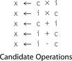 |
When
Process identifies
n as a candidate operation, it finds both the induction variable,
iv and the region constant,
rc.
DFS passes each
scc to
Process. If the
scc consists of a single node
n that has the form of a candidate operation, shown in the margin,
Process passes
n to
Replace, along with its induction variable,
iv, and its region constant,
rc.
Replace rewrites the code, as described in the next section. If the
scc contains multiple nodes,
Process passes the
scc to
ClassifyIV to determine whether or not it is an induction variable.
ClassifyIV examines each node in the
scc to check it against the set of valid updates for an induction variable. If all the updates are valid, the
scc is an induction variable, and
Process sets each node's header field to contain the node in the
scc with the lowest reverse postorder number. If the
scc is not an induction variable,
ClassifyIV revisits each node in the
scc to test it as a candidate operation, either passing it to
Replace or setting its header to show that it is not an induction variable.
Rewriting the Code
The remaining piece of
OSR implements the rewriting step. Both
Process and
ClassifyIV call
Replace to perform the rewrite. Figure 10.14 shows the code for
Replace and its support functions
Reduce and
Apply.
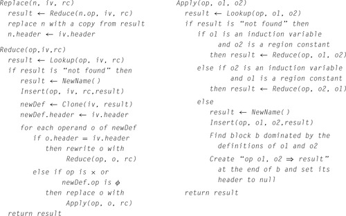
Replace takes three arguments, an
ssa graph node
n, an induction variable
iv, and a region constant
rc. The latter two are operands to
n.
Replace calls
Reduce to rewrite the operation represented by
n. Next, it replaces
n with a copy operation from the result produced by
Replace. It sets
n's header field, and returns.
Reduce and
Apply do most of the work. They use a hash table to avoid inserting duplicate operations. Since
OSR works on
ssa names, a single global hash table suffices. It can be initialized in
OSR before the first call to
DFS.
Insert adds entries to the hash table;
Lookup queries the table.
The plan for
Reduce is simple. It takes an opcode and its two operands and either creates a new induction variable to replace the computation or returns the name of an induction variable previously created for the same combination of opcode and operands. It consults the hash table to avoid duplicate work. If the desired induction variable is not in the hash table, it creates the induction variable in a two-step process. First, it calls
Clone to copy the definition for
iv, the induction variable in the operation being reduced. Next, it recurs on the operands of this new definition.
These operands fall into two categories. If the operand is defined inside the
scc, it is part of
iv, so
Reduce recurs on that operand. This forms the new induction variable by cloning its way around the
scc of the original induction variable
iv. An operand defined outside the
scc must be either the initial value of
iv or a value by which
iv is incremented. The initial value must be a
ϕ-function argument from outside the
scc;
Reduce calls
Apply on each such argument.
Reduce can leave an induction-variable increment alone, unless the candidate operation is a multiply. For a multiply,
Reduce must compute a new increment as the product of the old increment and the original region constant
rc. It invokes
Apply to generate this computation.
Apply takes an opcode and two operands, locates an appropriate point in the code, and inserts that operation. It returns the new
ssa name for the result of that operation. A few details need further explanation. If this new operation is, itself, a candidate,
Apply invokes
Reduce to handle it. Otherwise,
Apply gets a new name, inserts the operation, and returns the result. (If both
o1 and
o2 are constant,
Apply can evaluate the operation and insert an immediate load.) It locates an appropriate block for the new operation using dominance information. Intuitively, the new operation must go into a block dominated by the blocks that define its operands. If one operand is a constant,
Apply can duplicate the constant in the block that defines the other operand. Otherwise, both operands must have definitions that dominate the header block, and one must dominate the other.
Apply can insert the operation immediately after this later definition.
Back to the Example
Consider what happens when
OSR encounters the example in Figure 10.12. Assume that it begins with the node labelled
r
s
2 and that it visits left children before right children. It recurs down the chain of operations that define
r
4, r
3, r
2, r
1, and r
i
1. At
r
i
1, it recurs on
r
i
2 and then
r
i
0. It finds the two single-node
sccs that contain the literal constant one. Neither is a candidate, so
Process marks them as noninduction variables by setting their headers to
null.
The first nontrivial
scc that
DFS discovers contains
r
i
1 and
r
i
2. All the operations are valid updates for an induction variable, so
ClassifyIV marks each node as an induction variable by setting its header field to point to the node with the lowest depth-first number in the
scc—the node for
r
i
1.
Now,
DFS returns to the node for
r
1. Its left child is an induction variable and its right child is a region constant, so it invokes
Reduce to create an induction variable. In this case,
r
1 is
r
i
1 − 1, so the induction variable has an initial value equal to one less than the initial value of the old induction variable, or zero. The increment is the same. Figure 10.15 shows the
scc that
Reduce and
Apply create, under the label “for
r
1.” Finally, the definition of
r
1 is replaced with a copy operation,
r
1 ← r
t
1. The copy operation is marked as an induction variable.

Next,
DFS discovers the
scc that consists of the node labelled
r
2.
Process discovers that it is a candidate because its left operand (the copy that now defines
r
1 is an induction variable and its right operand is a region constant.
Process invokes
Replace to create an induction variable that has the value r
1 × 4.
Reduce and
Apply clone the induction variable for
r
1, adjust the increment since the operation is a multiply, and add a copy to
r
2.
DFS next passes the node for
r
3 to
Process. This creates another induction variable with
@a as its initial value and copies its value to
r
3.
Process handles the
load, followed by the
scc that computes the sum. It finds that none of these operations are candidates.
Finally,
OSR invokes
DFS on the unvisited node for the
cbr.
DFS visits the comparison, the previously marked induction variable, and the constant 100. No further reductions occur.
The
ssa graph in Figure 10.15 shows all of the induction variables created by this process. The induction variables labelled “for
r
1” and “for
r
2” are dead. The induction variable for
i would be dead, except that the end-of-loop test still uses it. To eliminate this induction variable, the compiler can apply linear-function test replacement to transfer the test to the induction variable for
r
3.
Linear-Function Test Replacement
Strength reduction often eliminates all uses of an induction variable, except for an end-of-loop test. In that case, the compiler may be able to rewrite the end-of-loop test to use another induction variable found in the loop. If the compiler can remove this last use, it can eliminate the original induction variable as dead code. This transformation is called linear-function test replacement (
lftr).
To perform
lftr, the compiler must (1) locate comparisons that rely on otherwise unneeded induction variables, (2) locate an appropriate new induction variable that the comparison could use, (3) compute the correct region constant for the rewritten test, and (4) rewrite the code. Having
lftr cooperate with
OSR can simplify all of these tasks to produce a fast, effective transformation.
The operations that
lftr targets compare the value of an induction variable against a region constant.
OSR examines each operation in the program to determine if it is a candidate for strength reduction. It can easily and inexpensively build a list of all the comparison operations that involve induction variables. After
OSR finishes its work,
lftr should revisit each of these comparisons. If the induction-variable argument of a comparison was strength reduced by
OSR,
lftr should retarget the comparison to use the new induction variable.
To facilitate this process,
Reduce can record the arithmetic relationship it uses to derive each new induction variable. It can insert a special
lftr edge from each node in the original induction variable to the corresponding node in its reduced counterpart and label it with the operation and region constant of the candidate operation responsible for creating that induction variable. Figure 10.16 shows the
ssa graph with these additional edges in black. The sequence of reductions in the example create a chain of labelled edges. Starting from the original induction variable, we find the labels
−1,
x4, and
+@a.
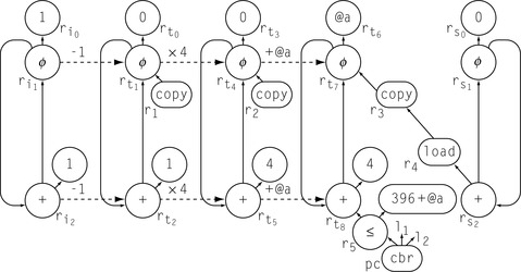
When
lftr finds a comparison that should be replaced, it can follow the edges from its induction-variable argument to the final induction variable that resulted from a chain of one or more reductions. The comparison should use this induction variable with an appropriate new region constant.
The labels on the
lftr edges describe the transformation that must be applied to the original region constant to derive the new region constant. In the example, the trail of edges leads from
r
i
2 to
r
t
8 and produces the value
(100 − 1) × 4, + @a for the transformed test. Figure 10.16 shows the edges and the rewritten test.
This version of
lftr is simple, efficient, and effective. It relies on close collaboration with
OSR to identify comparisons that might be retargeted and to record the reductions as it applies them. Using these two data structures,
lftr can find comparisons to retarget, find the appropriate place to retarget them, and find the necessary transformation for the comparison's constant argument.
10.7.3. Choosing an Optimization Sequence
Optimization Sequence
a set of optimizations and an order for their application
The effectiveness of an optimizer on any given code depends on the sequence of optimizations that it applies to the code—both the specific transformations that it uses and the order in which it applies them. Traditional optimizing compilers have offered the user the choice of several sequences (e.g.
−O, −O1, −O2, …). Those sequences provide a tradeoff between compile time and the amount of optimization that the compiler attempts. Increased optimization effort, however, does not guarantee improvement.
The optimization sequence problem arises because the effectiveness of any given transformation depends on several factors.
1. Does the opportunity that the transformation targets appear in the code? If not, the transformation cannot improve the code.
2. Has a prior transformation hidden or obscured that opportunity? For example, the optimization of algebraic identities in
lvn can convert
2 × a into a shift operation, which replaces a commutative operation with a faster non-commutative optimization. Any transformation that needs commutativity to effect its improvement might see opportunities vanish from prior application of
lvn.
3. Has any other transformation already eliminated the inefficiency? Transformations have overlapping and idiosyncratic effects; for example,
lvn achieves some of the effects of global constant propagation and loop unrolling achieves effects similar to superblock cloning. The compiler writer might include both transformations for their nonoverlapping effects.
The interactions between transformations makes it difficult to predict the improvement from the application of any single transformation or any sequence of transformations.
Some research compilers attempt to discover good optimization sequences. The approaches vary in granularity and in technique. The various systems have looked for sequences at the block level, at the source-file level, and at the whole-program level. Most of these systems have used some kind of search over the space of optimization sequences.
The space of potential optimization sequences is huge. For example, if the compiler chooses a sequence of length 10 from a pool of 15 transformations, it has 10
15 possible sequences that it can generate—an impractically large number for the compiler to explore. Thus, compilers that search for good sequences use heuristic techniques to sample smaller portions of the search space. In general, these techniques fall into three categories: (1) genetic algorithms adapted to act as intelligent searches, (2) randomized search algorithms, and (3) statistical machine learning techniques. All three approaches have shown promise.
In this context, a
good sequence is one that produces results within 5% of the best results.
Despite the huge size of the search spaces, well-tuned search algorithms can find good optimization sequences with 100 to 200 probes of the search space. While that number is not yet practical, further refinement may reduce the number of probes to a practical level.
One interesting application of these techniques is to derive the sequences used by the compiler's command line flags, such as
−O2. The compiler writer can use an ensemble of representative applications to discover good general sequences and then apply those sequences as the compiler's default sequences. A more aggressive approach, used in several systems, is to derive a handful of good sequences for different application ensembles and have the compiler try each of those sequences and retain the best result.
10.8. Summary and Perspective
The design and implementation of an optimizing compiler is a complex undertaking. This chapter has introduced a conceptual framework for thinking about transformations—the taxonomy of effects. Each category in the taxonomy is represented by several examples, either in this chapter or elsewhere in the book.
Chapter Notes
While the algorithms presented in this chapter are modern, many of the basic ideas were well known in the 1960s and 1970s. Dead-code elimination, code motion, strength reduction, and redundancy elimination are all described by Allen [11] and by Cocke and Schwartz [91]. A number of survey papers provide overviews of the state of the field at different points in time [16], [28], [30] and [316]. Books by Morgan [268] and Muchnick [270] both discuss the design, structure, and implementation of optimizing compilers. Wolfe [352] and Allen and Kennedy [20] focus on dependence-based analysis and transformations.
Dead implements a mark-sweep style of dead-code elimination that was introduced by Kennedy [215] and [217]. It is reminiscent of the Schorr-Waite marking algorithm [309].
Dead is specifically adapted from the work of Cytron et al. [110, Section 7.1].
Clean was developed and implemented in 1992 by Rob Shillner [254].
lcm improves on Morel and Renvoise's classic algorithm for partial redundancy elimination [267]. That paper inspired many improvements, including [81], [130], [133] and [321]. Knoop, Rüthing, and Steffen's
lcm[225] improved code placement; the formulation in Section 10.3 uses equations from Drechsler and Stadel [134]. Bodik, Gupta, and Soffa combined this approach with replication to find and remove all redundant code [43]. The
dvnt algorithm is due to Briggs [53]. It has been implemented in a number of compilers.
Hoisting appears in the Allen-Cocke catalogue as a technique for reducing code space [16]. The formulation using anticipability appears in several places, including Fischer and LeBlanc [147]. Sinking or cross-jumping is described by Wulf et al. [356].
Both peephole optimization and tail-recursion elimination date to the early 1960s. Peephole optimization was first described by McKeeman [260]. Tailrecursion elimination is older; folklore tells that McCarthy described it at the chalkboard during a talk in 1963. Steele's thesis [323] is a classic reference for tail-recursion elimination.
Superblock cloning was introduced by Hwu et al. [201]. Loop optimizations such as unswitching and unrolling have been studied extensively [20] and [28]; Kennedy used unrolling to avoid copy operations at the end of a loop [214]. Cytron, Lowrey, and Zadeck present an interesting alternative to unswitching [111]. McKinley et al. give practical insight into the impact of memory optimizations on performance [94] and [261].
Combining optimizations, as in
sccp, often leads to improvements that cannot be obtained by independent application of the original optimizations. Value numbering combines redundancy elimination, constant propagation, and simplification of algebraic identities [53].
lcm combines elimination of redundancies and partial redundancies with code motion [225]. Click and Cooper [86] combine Alpern's partitioning algorithm [21] with
sccp[347]. Many authors have combined register allocation and instruction scheduling [48], [163], [269], [276], [277], [285] and [308].
The
sccp algorithm is due to Wegman and Zadeck [346] and [347]. Their work clarified the distinction between optimistic and pessimistic algorithms; Click discusses the same issue from a set-building perspective [84].
Operator strength reduction has a rich history. One family of strengthreduction algorithms developed out of work by Allen, Cocke, and Kennedy [19], [88], [90], [216] and [256]. The
OSR algorithm is in this family [107]. Another family of algorithms grew out of the data-flow approach to optimization exemplified by the
lcm algorithm; a number of sources give techniques in this family [127], [129], [131], [178], [209], [220] and [226]. The version of
OSR in Section 10.7.2 only reduces multiplications. Allen et al. show the reduction sequences for many other operators [19]; extending
OSR to handle these cases is straightforward. A weaker form of strength reduction rewrites integer multiplies with faster operations [243].
Section 10.1
1. One of the primary functions of an optimizer is to remove overhead that the compiler introduced during the translation from source language into
ir.
a. Give four examples of inefficiencies that you would expect an optimizer to improve, along with the source-language constructs that give rise to them.
b. Give four examples of inefficiencies that you would expect an optimizer to miss, even though they can be improved. Explain why an optimizer would have difficulty improving them.
Section 10.2
2. Figure 10.1 shows the algorithm for
Dead. The marking pass is a classic fixed-point computation.
a. Explain why this computation terminates.
b. Is the fixed-point that it finds unique? Prove your answer.
c. Derive a tight time bound for the algorithm.
3. Consider the algorithm
Clean from Section 10.2. It removes useless control flow and simplifies the
cfg.
a. Why does the algorithm terminate?
b. Give an overall time bound for the algorithm.
Section 10.3
4.
lcm uses data-flow analysis to find redundancy and to perform code motion. Thus, it relies on a lexical notion of identity to find redundancy—two expressions can only be redundant if the data-flow analysis maps them to the same internal name. By contrast, value numbering computes identity based on values.
a. Give an example of a redundant expression that
lcm will discover but a value-based algorithm (say a global version of value numbering) will not.
b. Give an example of a redundant expression that
lcm will not discover but a value-based algorithm will.
5. Redundancy elimination has a variety of effects on the code that the compiler generates.
a. How does
lcm affect the demand for registers in the code being transformed? Justify your answer.
b. How does
lcm affect the size of the code generated for a procedure? (You can assume that demand for registers is unchanged.)
c. How does hoisting affect the demand for registers in the code being transformed? Justify your answer.
d. How does hoisting affect the size of the code generated for a procedure? (Use the same assumptions.)
Section 10.4
6. A simple form of operator strength reduction replaces a single instance of an expensive operation with a sequence of operations that are less expensive to execute. For example, some integer multiply operations can be replaced with a sequence of shifts and adds.
a. What conditions must hold to let the compiler safely replace an integer operation
x ← y × z with a single shift operation?
b. Sketch an algorithm that replaces a multiplication of a known constant and an unsigned integer with a sequence of shifts and adds in cases where the constant is not a power of two.
7. Both tail-call optimization and inline substitution attempt to reduce the overhead caused by the procedure linkage.
a. Can the compiler inline a tail call? What obstacles arise? How might you work around them?
b. Contrast the code produced from your modified inlining scheme with that produced by tail-call optimization.
Section 10.5
8. A compiler can find and eliminate redundant computations in many different ways. Among these are
dvnt and
lcm.
a. Give two examples of redundancies eliminated by
dvnt that cannot be found by
lcm.
b. Give an example that
lcm finds that is missed by
dvnt.
Section 10.6
9. Develop an algorithm to rename the value in a procedure to that encodes value identity into variable names.
10. Superblock cloning can cause significant code growth.
Hint: Think back to the block-placement algorithm in Chapter 8.
a. How might the compiler mitigate code growth in superblock cloning while retaining as much of the benefit as possible?
b. What problems might arise if the optimizer allowed superblock cloning to continue across a loop-closing branch? Contrast your approach with loop unrolling.
..................Content has been hidden....................
You can't read the all page of ebook, please click here login for view all page.