Chapter 3
Linear Block Codes
3.1 Basic Definitions
Consider a source that produces symbols from an alphabet ![]() having
having ![]() symbols, where
symbols, where ![]() forms a field. We refer to a tuple
forms a field. We refer to a tuple ![]() with
with ![]() elements as an
elements as an ![]() ‐vector or an
‐vector or an ![]() ‐tuple.
‐tuple.
For a block code to be useful for error correction purposes, there should be a one‐to‐one correspondence between a message ![]() and its codeword
and its codeword ![]() . However, for a given code
. However, for a given code ![]() , there may be more than one possible way of mapping messages to codewords.
, there may be more than one possible way of mapping messages to codewords.
A block code can be represented as an exhaustive list, but for large ![]() this would be prohibitively complex to store and decode. The complexity can be reduced by imposing some sort of mathematical structure on the code. The most common requirement is linearity.
this would be prohibitively complex to store and decode. The complexity can be reduced by imposing some sort of mathematical structure on the code. The most common requirement is linearity.
In some literature, an ![]() linear code is denoted using square brackets,
linear code is denoted using square brackets, ![]() . A linear code may also be designated as
. A linear code may also be designated as ![]() , where
, where ![]() is the minimum distance of the code (as discussed below).
is the minimum distance of the code (as discussed below).
For a linear code, the sum of any two codewords is also a codeword. More generally, any linear combination of codewords is a codeword.
Recall from Definition 1.11 that the minimum distance is the smallest Hamming distance between any two codewords of the code.
An ![]() code with minimum distance
code with minimum distance ![]() is sometimes denoted as an
is sometimes denoted as an ![]() code.
code.
As described in Section 1.8.1, the random error correcting capability of a code with minimum distance ![]() is
is ![]() .
.
3.2 The Generator Matrix Description of Linear Block Codes
Since a linear block code ![]() is a
is a ![]() ‐dimensional vector space, there exist
‐dimensional vector space, there exist ![]() linearly independent vectors which we designate as
linearly independent vectors which we designate as ![]() such that every codeword
such that every codeword ![]() in
in ![]() can be represented as a linear combination of these vectors,
can be represented as a linear combination of these vectors,
where ![]() . (For binary codes, all arithmetic in 3.1 is done modulo 2; for codes of
. (For binary codes, all arithmetic in 3.1 is done modulo 2; for codes of ![]() , the arithmetic is done in
, the arithmetic is done in ![]() .) Thinking of the
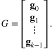
.) Thinking of the ![]() as row vectors1 and stacking up, we form the
as row vectors1 and stacking up, we form the ![]() matrix
matrix ![]() ,
,
Let
Then 3.1 can be written as
and every codeword ![]() has such a representation for some vector
has such a representation for some vector ![]() . Since the rows of
. Since the rows of ![]() generate (or span) the
generate (or span) the ![]() linear code
linear code ![]() ,
, ![]() is called a generator matrix for
is called a generator matrix for ![]() . Equation 3.2 can be thought of as an encoding operation for the code
. Equation 3.2 can be thought of as an encoding operation for the code ![]() . Representing the code thus requires storing only
. Representing the code thus requires storing only ![]() vectors of length
vectors of length ![]() (rather than the
(rather than the ![]() vectors that would be required to store all codewords of a nonlinear code).
vectors that would be required to store all codewords of a nonlinear code).
Note that the representation of the code provided by ![]() is not unique. From a given generator
is not unique. From a given generator ![]() , another generator
, another generator ![]() can be obtained by performing row operations (nonzero linear combinations of the rows). Then an encoding operation defined by
can be obtained by performing row operations (nonzero linear combinations of the rows). Then an encoding operation defined by ![]() maps the message
maps the message ![]() to a codeword in
to a codeword in ![]() , but it is not necessarily the same codeword that would be obtained using the generator
, but it is not necessarily the same codeword that would be obtained using the generator ![]() .
.
It should be emphasized that being systematic is a property of the encoder and not a property of the code. For a linear block code, the encoding operation represented by ![]() is systematic if an identity matrix can be identified among the rows of
is systematic if an identity matrix can be identified among the rows of ![]() . Neither the generator
. Neither the generator ![]() nor
nor ![]() of Example 3.5 are systematic.
of Example 3.5 are systematic.
Frequently, a systematic generator is written in the form

where ![]() is the
is the ![]() identity matrix and
identity matrix and ![]() is a
is a ![]() matrix which generates parity symbols. The encoding operation is
matrix which generates parity symbols. The encoding operation is
The codeword is divided into two parts: the part ![]() consists of the message symbols, and the part
consists of the message symbols, and the part ![]() consists of the parity check symbols.
consists of the parity check symbols.
Performing elementary row operations (replacing a row with linear combinations of some rows) does not change the row span, so that the same code is produced. If two columns of a generator are interchanged, then the corresponding positions of the code are changed, but the distance structure of the code is preserved.
Let ![]() and
and ![]() be generator matrices of equivalent codes. Then
be generator matrices of equivalent codes. Then ![]() and
and ![]() are related by the following operations:
are related by the following operations:
- Column permutations,
- Elementary row operations.
Given an arbitrary generator ![]() , it is possible to put it into the form 3.4 by performing Gaussian elimination with pivoting.
, it is possible to put it into the form 3.4 by performing Gaussian elimination with pivoting.
3.2.1 Rudimentary Implementation
Implementing encoding operations for binary codes is straightforward, since the multiplication operation corresponds to the
and
operation and the addition operation corresponds to the
exclusive‐or
operation. For software implementations, encoding is accomplished by straightforward matrix/vector multiplication. This can be greatly accelerated for binary codes by packing several bits into a single word (e.g., 32 bits in an
unsigned int
of 4 bytes). The multiplication is then accomplished using the bit
exclusive‐or
operation of the language (e.g., the
^
operator of C). Addition must be accomplished by looping through the bits, or by precomputing bit sums and storing them in a table, where they can be immediately looked up.
3.3 The Parity Check Matrix and Dual Codes
Since a linear code ![]() is a
is a ![]() ‐dimensional vector subspace of
‐dimensional vector subspace of ![]() , by Theorem 2.64 there must be a dual space to
, by Theorem 2.64 there must be a dual space to ![]() of dimension
of dimension ![]() .
.
As a vector space, ![]() has a basis which we denote by
has a basis which we denote by ![]() . We form a matrix
. We form a matrix ![]() using these basis vectors as rows:
using these basis vectors as rows:
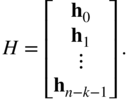
This matrix is known as the parity check matrix for the code ![]() . The generator matrix and the parity check matrix for a code satisfy
. The generator matrix and the parity check matrix for a code satisfy
The parity check matrix has the following important property:
(Sometimes additional linearly dependent rows are included in ![]() , but the same result still holds.)
, but the same result still holds.)
When ![]() is in systematic form 3.4, a parity check matrix is readily determined:
is in systematic form 3.4, a parity check matrix is readily determined:
(For the field ![]() ,
, ![]() , since 1 is its own additive inverse.) Frequently, a parity check matrix for a code is obtained by finding a generator matrix in systematic form and employing (3.6).
, since 1 is its own additive inverse.) Frequently, a parity check matrix for a code is obtained by finding a generator matrix in systematic form and employing (3.6).
The condition ![]() imposes linear constraints among the bits of
imposes linear constraints among the bits of ![]() called the parity check equations.
called the parity check equations.
A parity check matrix for a code (whether systematic or not) provides information about the minimum distance of the code.
3.3.1 Some Simple Bounds on Block Codes
Theorem 3.13 leads to a relationship between ![]() ,
, ![]() , and
, and ![]() :
:
Note: Although this bound is proved here for linear codes, it is also true for nonlinear codes. (See [292].)
A code for which ![]() is called a maximum distance separable (MDS) code.
is called a maximum distance separable (MDS) code.
Thinking geometrically, around each code point is a cloud of points corresponding to non‐codewords. (See Figure 1.17.) For a ![]() ‐ary code, there are
‐ary code, there are ![]() vectors at a Hamming distance 1 away from a codeword,
vectors at a Hamming distance 1 away from a codeword, ![]() vectors at a Hamming distance 2 away from a codeword and, in general,
vectors at a Hamming distance 2 away from a codeword and, in general, ![]() vectors at a Hamming distance
vectors at a Hamming distance ![]() from a codeword.
from a codeword.
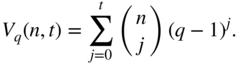
The vectors at Hamming distances ![]() away from a codeword form a “sphere” called the Hamming sphere of radius
away from a codeword form a “sphere” called the Hamming sphere of radius ![]() . The number of vectors in a Hamming sphere up to radius
. The number of vectors in a Hamming sphere up to radius ![]() for a code of length
for a code of length ![]() over an alphabet of
over an alphabet of ![]() symbols is denoted
symbols is denoted ![]() , where
, where

The bounded distance decoding sphere of a codeword is the Hamming sphere of radius ![]() around the codeword. Equivalently, a code whose random error correction capability is
around the codeword. Equivalently, a code whose random error correction capability is ![]() must have a minimum distance between codewords satisfying
must have a minimum distance between codewords satisfying ![]() .
.
The redundancy of a code is essentially the number of parity symbols in a codeword. More precisely we have
where ![]() is the number of codewords. For a linear code we have
is the number of codewords. For a linear code we have ![]() , so
, so ![]() .
.
A code satisfying the Hamming bound with equality is said to be a perfect code. Actually, being perfect codes does not mean the codes are the best possible codes; it is simply a designation regarding how points fall in the Hamming spheres. The set of perfect codes is actually quite limited. It has been proved (see [292]) that the entire set of perfect codes is:
- The set of all
 ‐tuples, with minimum distance = 1 and
  .
. - Odd‐length binary repetition codes.
- Binary and nonbinary Hamming codes (linear) or other nonlinear codes with equivalent parameters.
- The binary
 Golay code
  .
. - The ternary (i.e., over
 )
)  code
code  and the (23,11,5) code
  . These codes are discussed in Chapter 8.
3.4 Error Detection and Correction Over Hard‐Output Channels
By Theorem 3.10, ![]() if and only if
if and only if ![]() is a codeword of
is a codeword of ![]() . In medical terminology, a syndrome is a pattern of symptoms that aids in diagnosis; here
. In medical terminology, a syndrome is a pattern of symptoms that aids in diagnosis; here ![]() aids in diagnosing if
aids in diagnosing if ![]() is a codeword or has been corrupted by noise. As we will see, it also aids in determining what the error is.
is a codeword or has been corrupted by noise. As we will see, it also aids in determining what the error is.
3.4.1 Error Detection
The syndrome can be used as an error detection scheme. Suppose that a codeword ![]() in a binary linear block code
in a binary linear block code ![]() over
over ![]() is transmitted through a hard channel (e.g., a binary code over a BSC) and that the
is transmitted through a hard channel (e.g., a binary code over a BSC) and that the ![]() ‐vector
‐vector ![]() is received. We can write
is received. We can write
where the arithmetic is done in ![]() , and where
, and where ![]() is the error vector, being 0 in precisely the locations where the channel does not introduce errors. The received vector
is the error vector, being 0 in precisely the locations where the channel does not introduce errors. The received vector ![]() could be any of the vectors in
could be any of the vectors in ![]() , since any error pattern is possible. Let
, since any error pattern is possible. Let ![]() be a parity check matrix for
be a parity check matrix for ![]() . Then the syndrome
. Then the syndrome
From Theorem 3.10, ![]() if
if ![]() is a codeword. However, if
is a codeword. However, if ![]() , then an error condition has been detected: we do not know what the error is, but we do know that an error has occurred. (Some additional perspective to this problem is provided in Box 3.1.)
, then an error condition has been detected: we do not know what the error is, but we do know that an error has occurred. (Some additional perspective to this problem is provided in Box 3.1.)
3.4.2 Error Correction: The Standard Array
Let us now consider one method of decoding linear block codes transmitted through a hard channel using maximum likelihood (ML) decoding. As discussed in Section 1.8.1, ML decoding of a vector ![]() consists of choosing the codeword
consists of choosing the codeword ![]() that is closest to
that is closest to ![]() in Hamming distance. That is,
in Hamming distance. That is,
Let the set of codewords in the code be ![]() , where
, where ![]() . Let us take
. Let us take ![]() , the all‐zero codeword. Let
, the all‐zero codeword. Let ![]() denote the set of
denote the set of ![]() ‐vectors which are closer to the codeword
‐vectors which are closer to the codeword ![]() than to any other codeword. (Vectors which are equidistant to more than one codeword are assigned into a set
than to any other codeword. (Vectors which are equidistant to more than one codeword are assigned into a set ![]() at random.) The sets
at random.) The sets ![]() partition the space of
partition the space of ![]() ‐vectors into
‐vectors into ![]() disjoint subsets. If
disjoint subsets. If ![]() falls in the set
falls in the set ![]() , then, being closer to
, then, being closer to ![]() than to any other codeword,
than to any other codeword, ![]() is decoded as
is decoded as ![]() . So, decoding can be accomplished if the
. So, decoding can be accomplished if the ![]() sets can be found.
sets can be found.
The standard array is a representation of the partition ![]() . It is a two‐dimensional array in which the columns of the array represent the
. It is a two‐dimensional array in which the columns of the array represent the ![]() . The standard array is built as follows. First, every codeword
. The standard array is built as follows. First, every codeword ![]() belongs in its own set
belongs in its own set ![]() . Writing down the set of codewords thus gives the first row of the array. From the remaining vectors in
. Writing down the set of codewords thus gives the first row of the array. From the remaining vectors in ![]() , find the vector
, find the vector ![]() of smallest weight. This must lie in the set
of smallest weight. This must lie in the set ![]() , since it is closest to the codeword
, since it is closest to the codeword ![]() . But
. But
for each ![]() , so the vector
, so the vector ![]() must also lie in
must also lie in ![]() for each
for each ![]() . So
. So ![]() is placed into each
is placed into each ![]() . The vectors
. The vectors ![]() are included in their respective columns of the standard array to form the second row of the standard array. The procedure continues, selecting an unused vector of minimal weight and adding it to each codeword to form the next row of the standard array, until all
are included in their respective columns of the standard array to form the second row of the standard array. The procedure continues, selecting an unused vector of minimal weight and adding it to each codeword to form the next row of the standard array, until all ![]() possible vectors have been used in the standard array. In summary:
possible vectors have been used in the standard array. In summary:
- Write down all the codewords of the code
 .
. - Select from the remaining unused vectors of
 one of minimal weight,
  . Write
  in the column under the all‐zero codeword, then add
  to each codeword in turn, writing the sum in the column under the corresponding codeword.
 - Repeat step 2 until all
 vectors in
  have been placed in the standard array.
Table 3.1 The Standard Array for a Code
| Row 1 | 0000000 | 0111100 | 1011010 | 1100110 | 1101001 | 1010101 | 0110011 | 0001111 |
|---|---|---|---|---|---|---|---|---|
| Row 2 | 1000000 | 1111100 | 0011010 | 0100110 | 0101001 | 0010101 | 1110011 | 1001111 |
| Row 3 | 0100000 | 0011100 | 1111010 | 1000110 | 1001001 | 1110101 | 0010011 | 0101111 |
| Row 4 | 0010000 | 0101100 | 1001010 | 1110110 | 1111001 | 1000101 | 0100011 | 0011111 |
| Row 5 | 0001000 | 0110100 | 1010010 | 1101110 | 1100001 | 1011101 | 0111011 | 0000111 |
| Row 6 | 0000100 | 0111000 | 1011110 | 1100010 | 1101101 | 1010001 | 0110111 | 0001011 |
| Row 7 | 0000010 | 0111110 | 1011000 | 1100100 | 1101011 | 1010111 | 0110001 | 0001101 |
| Row 8 | 0000001 | 0111101 | 1011011 | 1100111 | 1101000 | 1010100 | 0110010 | 0001110 |
| Row 9 | 1100000 | 1011100 | 0111010 | 0000110 | 0001001 | 0110101 | 1010011 | 1101111 |
| Row 10 | 1010000 | 1101100 | 0001010 | 0110110 | 0111001 | 0000101 | 1100011 | 1011111 |
| Row 11 | 0110000 | 0001100 | 1101010 | 1010110 | 1011001 | 1100101 | 0000011 | 0111111 |
| Row 12 | 1001000 | 1110100 | 0010010 | 0101110 | 0100001 | 0011101 | 1111011 | 1000111 |
| Row 13 | 0101000 | 0010100 | 1110010 | 1001110 | 1000001 | 1111101 | 0011011 | 0100111 |
| Row 14 | 0011000 | 0100100 | 1000010 | 1111110 | 1110001 | 1001101 | 0101011 | 0010111 |
| Row 15 | 1000100 | 1111000 | 0011110 | 0100010 | 0101101 | 0010001 | 1110111 | 1001011 |
| Row 16 | 1110000 | 1001100 | 0101010 | 0010110 | 0011001 | 0100101 | 1000011 | 1111111 |
The horizontal lines in the standard array separate the error patterns of different weights.
We make the following observations:
- There are
 codewords (columns) and
  possible vectors, so there are
  rows in the standard array. We observe, therefore, that: an
  code is capable of correcting
  different error patterns.
 - The difference (or sum, over
 ) of any two vectors in the same row of the standard array is a code vector. In a row, the vectors are
  and
and  . Then
which is a codeword, since linear codes form a vector subspace.
. Then
which is a codeword, since linear codes form a vector subspace.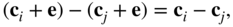
- No two vectors in the same row of a standard array are identical. Because otherwise we have
which means
 , which is impossible.
 - Every vector appears exactly once in the standard array. We know every vector must appear at least once, by the construction. If a vector appears in both the
 th row and the
  th row, we must have
for some
th row, we must have
for some
 and
and  . Let us take
  . We have
for some
. We have
for some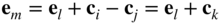
 . This means that
  is on the
  th row of the array, which is a contradiction.
The rows of the standard array are called cosets. Each row is of the form
That is, the rows of the standard array are translations of ![]() . These are the same cosets we met in Section 2.2.3 in conjunction with groups.
. These are the same cosets we met in Section 2.2.3 in conjunction with groups.
The vectors in the first column of the standard array are called the coset leaders. They represent the error patterns that can be corrected by the code under this decoding strategy. The decoder of Example 3.19 is capable of correcting all errors of weight 1, seven different error patterns of weight 2, and one error pattern of weight 3.
To decode with the standard array, we first locate the received vector ![]() in the standard array. Then identify
in the standard array. Then identify
for a vector ![]() which is a coset leader (in the left column) and a codeword
which is a coset leader (in the left column) and a codeword ![]() (on the top row). Since we designed the standard array with the smallest error patterns as coset leaders, the error codeword so identified in the standard array is the ML decision. The coset leaders are called the correctable error patterns.
(on the top row). Since we designed the standard array with the smallest error patterns as coset leaders, the error codeword so identified in the standard array is the ML decision. The coset leaders are called the correctable error patterns.
As this decoding example shows, the standard array decoder may have coset leaders with weight higher than the random‐error‐correcting capability of the code ![]() .
.
This observation motivates the following definition.
If a standard array is used as the decoding mechanism, then complete decoding is achieved. On the other hand, if the rows of the standard array are filled out so that all instances of up to ![]() errors appear in the table, and all other rows are left out, then a bounded distance decoder is obtained.
errors appear in the table, and all other rows are left out, then a bounded distance decoder is obtained.
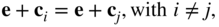
A perfect code can be understood in terms of the standard array: it is one for which there are no “leftover” rows: for binary codes all ![]() error patterns of weight
error patterns of weight ![]() and all lighter error patterns appear as coset leaders in the table, with no “leftovers.” (For
and all lighter error patterns appear as coset leaders in the table, with no “leftovers.” (For ![]() ‐ary codes, the number of error patterns is
‐ary codes, the number of error patterns is ![]() .)
.)
What makes it “perfect” then, is that the bounded distance decoder is also the ML decoder.
The standard array can, in principle, be used to decode any linear block code, but suffers from a major problem: the memory required to represent the standard array quickly become excessive, and decoding requires searching the entire table to find a match for a received vector ![]() . For example, a
. For example, a ![]() binary code — not a particularly long code by modern standards — would require
binary code — not a particularly long code by modern standards — would require ![]() vectors of length 256 bits to be stored in it and every decoding operation would require on average searching through half of the table.
vectors of length 256 bits to be stored in it and every decoding operation would require on average searching through half of the table.
A first step in reducing the storage and search complexity (which doesn't go far enough) is to use syndrome decoding. Let ![]() be a vector in the standard array. The syndrome for this vector is
be a vector in the standard array. The syndrome for this vector is ![]() . Furthermore, every vector in the coset has the same syndrome:
. Furthermore, every vector in the coset has the same syndrome: ![]() . We therefore only need to store syndromes and their associated error patterns. This table is called the syndrome decoding table. It has
. We therefore only need to store syndromes and their associated error patterns. This table is called the syndrome decoding table. It has ![]() rows but only two columns, so it is smaller than the entire standard array. But is still impractically large in many cases.
rows but only two columns, so it is smaller than the entire standard array. But is still impractically large in many cases.
With the syndrome decoding table, decoding is done as follows:
- Compute the syndrome,
 .
. - In the syndrome decoding table look up the error pattern
 corresponding to
  .
. - Then
 .
.
Despite the significant reduction compared to the standard array, the memory requirements for the syndrome decoding table are still very high. It is still infeasible to use this technique for very long codes. Additional algebraic structure must be imposed on the code to enable decoding long codes.
3.5 Weight Distributions of Codes and Their Duals
The weight distribution of a code plays a significant role in calculating probabilities of error.
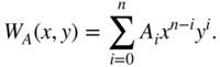
The weight enumerator is (essentially) the ![]() ‐transform of the weight distribution sequence.
‐transform of the weight distribution sequence.
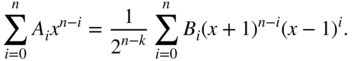
There is a relationship, known as the MacWilliams identities, between the weight enumerator of a linear code and its dual. This relationship is of interest because for many codes it is possible to directly characterize the weight distribution of the dual code, from which the weight distribution of the code of interest is obtained by the MacWilliams identity.
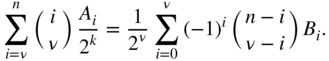
For binary codes with ![]() , the MacWilliams identities are
, the MacWilliams identities are

The proof of this theorem reveals some techniques that are very useful in coding. We give the proof for codes over ![]() , but it is straightforward to extend to larger fields (once you are familiar with them). The proof relies on the Hadamard transform. For a function
, but it is straightforward to extend to larger fields (once you are familiar with them). The proof relies on the Hadamard transform. For a function ![]() defined on
defined on ![]() , the Hadamard transform
, the Hadamard transform ![]() of
of ![]() is
is

where the sum is taken over all ![]()
![]() ‐tuples
‐tuples ![]() , where each
, where each ![]() . The inverse Hadamard transform is
. The inverse Hadamard transform is

3.6 Binary Hamming Codes and Their Duals
We now formally introduce a family of binary linear block codes, the Hamming codes, and their duals.
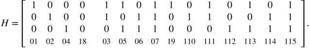
For example, when ![]() , we get
, we get

as the parity check matrix for a ![]() Hamming code. However, it is usually convenient to reorder the columns — resulting in an equivalent code — so that the identity matrix which is interspersed throughout the columns of
Hamming code. However, it is usually convenient to reorder the columns — resulting in an equivalent code — so that the identity matrix which is interspersed throughout the columns of ![]() appears in the first
appears in the first ![]() columns. We therefore write
columns. We therefore write
It is clear from the form of the parity check matrix that for any ![]() there exist three columns which add to zero; for example,
there exist three columns which add to zero; for example,

so by Theorem 3.13 the minimum distance is 3; Hamming codes are capable of correcting 1 bit error in the block, or detecting up to 2 bit errors.
An algebraic decoding procedure for Hamming codes was described in Section 1.9.1.
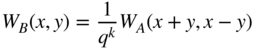
The dual to a ![]() Hamming code is a
Hamming code is a ![]() code called a simplex code or a maximal‐length feedback shift register code.
code called a simplex code or a maximal‐length feedback shift register code.
In general, all of the nonzero codewords of the ![]() simplex code have weight
simplex code have weight ![]() (see Exercise 3.12) and every pair of codewords is at a distance
(see Exercise 3.12) and every pair of codewords is at a distance ![]() apart (which is why it is called a simplex). For example, for the
apart (which is why it is called a simplex). For example, for the ![]() case, the codewords
case, the codewords ![]() form a tetrahedron. Thus, the weight enumerator of the dual code is
form a tetrahedron. Thus, the weight enumerator of the dual code is
From the weight enumerator of the dual, we find using (3.13) that the weight distribution of the Hamming code is
3.7 Performance of Linear Codes
There are several different ways that we can characterize the error detecting and correcting capabilities of codes at the output of the channel decoder [483].
 is the probability of decoder error, also known as the word error rate. This is the probability that the codeword at the output of the decoder is not the same as the codeword at the input of the encoder.
  or
or  is the probability of bit error, also known as the bit error rate. This is the probability that the decoded message bits (extracted from a decoded codeword of a binary code) are not the same as the encoded message bits. Note that when a decoder error occurs, there may be anywhere from 1 to
  message bits in error, depending on what codeword is sent, what codeword was decoded, and the mapping from message bits to codewords.
  is the probability of undetected codeword error, the probability that errors occurring in a codeword are not detected.
  is the probability of detected codeword error, the probability that one or more errors occurring in a codeword are detected.
  is the undetected bit error rate, the probability that a decoded message bit is in error and is contained within a codeword corrupted by an undetected error.
  is the detected bit error rate, the probability that a received message bit is in error and is contained within a codeword corrupted by a detected error.
  is the probability of decoder failure, which is the probability that the decoder is unable to decode the received vector (e.g., for a bounded distance decoder) and is able to determine that it cannot decode.
In what follows, bounds and exact expressions for these probabilities will be developed.
3.7.1 Error Detection Performance
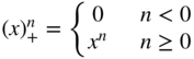
All errors with weight up to ![]() can be detected, so in computing the probability of detection, only error patterns with weight
can be detected, so in computing the probability of detection, only error patterns with weight ![]() or higher need be considered. If a codeword
or higher need be considered. If a codeword ![]() of a linear code is transmitted and the error pattern
of a linear code is transmitted and the error pattern ![]() happens to be a codeword,
happens to be a codeword, ![]() , then the received vector
, then the received vector
is also a codeword. Hence, the error pattern would be undetectable. Thus, the probability that an error pattern is undetectable is precisely the probability that it is a codeword.
We consider only errors in transmission of binary codes over the BSC with crossover probability ![]() . (Extension to codes with larger alphabets is discussed in [483].) The probability of any particular pattern of
. (Extension to codes with larger alphabets is discussed in [483].) The probability of any particular pattern of ![]() errors in a codeword is
errors in a codeword is ![]() . Recalling that
. Recalling that ![]() is the number of codewords in
is the number of codewords in ![]() of weight
of weight ![]() , the probability that
, the probability that ![]() errors form a codeword is
errors form a codeword is ![]() . The probability of undetectable error in a codeword is then
. The probability of undetectable error in a codeword is then

The probability of a detected codeword error is the probability that one or more errors occur minus the probability that the error is undetected:
Computing these probabilities requires knowing the weight distribution of the code, which is not always available. It is common, therefore, to provide bounds on the performance. A bound on ![]() can be obtained by observing that the probability of undetected error is bounded above by the probability of occurrence of any error patterns of weight greater than or equal to
can be obtained by observing that the probability of undetected error is bounded above by the probability of occurrence of any error patterns of weight greater than or equal to ![]() . Since there are
. Since there are ![]() different ways that
different ways that ![]() positions out of
positions out of ![]() can be changed,
can be changed,

A bound on ![]() is simply
is simply
The corresponding bit error rates can be bounded as follows. The undetected bit error rate ![]() can be lower‐bounded by assuming the undetected codeword error corresponds to only a single message bit error.
can be lower‐bounded by assuming the undetected codeword error corresponds to only a single message bit error. ![]() can be upper‐bounded by assuming that the undetected codeword error corresponds to all
can be upper‐bounded by assuming that the undetected codeword error corresponds to all ![]() message bits being in error. Thus,
message bits being in error. Thus,
Similarly for ![]() :
:
3.7.2 Error Correction Performance
An error pattern is correctable if and only if it is a coset leader in the standard array for the code, so the probability of correcting an error is the probability that the error is a coset leader. Let ![]() denote the number of coset leaders of weight
denote the number of coset leaders of weight ![]() . The numbers
. The numbers ![]() are called the coset leader weight distribution. Over a BSC with crossover probability
are called the coset leader weight distribution. Over a BSC with crossover probability ![]() , the probability of
, the probability of ![]() errors forming one of the coset leaders is
errors forming one of the coset leaders is ![]() . The probability of a decoding error is thus the probability that the error is not one of the coset leaders
. The probability of a decoding error is thus the probability that the error is not one of the coset leaders
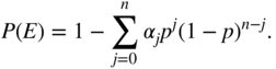
This result applies to any linear code with a complete decoder.
Most hard‐decision decoders are bounded‐distance decoders, selecting the codeword ![]() which lies within a Hamming distance of
which lies within a Hamming distance of ![]() of the received vector
of the received vector ![]() . An exact expression for the probability of error for a bounded‐distance decoder can be developed as follows. Let
. An exact expression for the probability of error for a bounded‐distance decoder can be developed as follows. Let ![]() be the probability that a received word
be the probability that a received word ![]() is exactly Hamming distance
is exactly Hamming distance ![]() from a codeword of weight
from a codeword of weight ![]() .
.
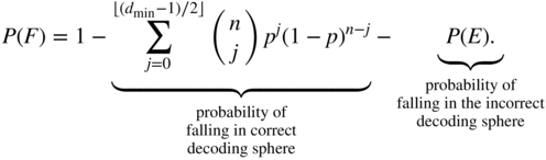
The probability of error is now obtained as follows.
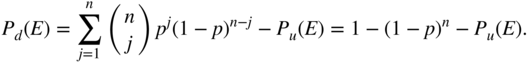
The probability of decoder failure for the bounded distance decoder is the probability that the received codeword does not fall into any of the decoding spheres,
Exact expressions to compute ![]() require information relating the weight of the message bits and the weight of the corresponding codewords. This information is summarized in the number
require information relating the weight of the message bits and the weight of the corresponding codewords. This information is summarized in the number ![]() , which is the total weight of the message blocks associated with codewords of weight
, which is the total weight of the message blocks associated with codewords of weight ![]() .
.
Modifying 3.21, we obtain

(See
hamcode74pe.m
.) Unfortunately, while obtaining values for ![]() for small codes is straightforward computationally, appreciably large codes require theoretical expressions which are usually unavailable.
for small codes is straightforward computationally, appreciably large codes require theoretical expressions which are usually unavailable.
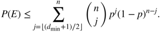
The probability of decoder error can be easily bounded by the probability of any error patterns of weight greater than ![]() :
:
An easy bound on probability of failure is the same as the bound on this probability of error.
Bounds on the probability of bit error can be obtained as follows. A lower bound is obtained by assuming that a decoder error causes a single bit error out of the ![]() message bits. An upper bound is obtained by assuming that all
message bits. An upper bound is obtained by assuming that all ![]() message bits are incorrect when the block is incorrectly decoded. This leads to the bounds
message bits are incorrect when the block is incorrectly decoded. This leads to the bounds
3.7.3 Performance for Soft‐Decision Decoding
While all of the decoding in this chapter has been for hard‐input decoders, it is interesting to examine the potential performance for soft‐decision decoding. Suppose the codewords of an ![]() code
code ![]() are modulated to a vector
are modulated to a vector ![]() using BPSK having energy
using BPSK having energy ![]() per coded bit and transmitted through an AWGN with variance
per coded bit and transmitted through an AWGN with variance ![]() . The transmitted vector
. The transmitted vector ![]() is a point in
is a point in ![]() ‐dimensional space. In Exercise 1.15, it is shown that the Euclidean distance between two BPSK modulated codewords is related to the Hamming distance between the codewords by
‐dimensional space. In Exercise 1.15, it is shown that the Euclidean distance between two BPSK modulated codewords is related to the Hamming distance between the codewords by
Suppose that there are ![]() codewords (on average) at a distance
codewords (on average) at a distance ![]() from a codeword. By the union bound (1.27), the probability of a block decoding error is given by
from a codeword. By the union bound (1.27), the probability of a block decoding error is given by

Neglecting the multiplicity constant ![]() , we see that we achieve essentially comparable performance compared to uncoded transmission when
, we see that we achieve essentially comparable performance compared to uncoded transmission when

The asymptotic coding gain is the factor by which the coded ![]() can be decreased to obtain equivalent performance. (It is called asymptotic because it applies only as the SNR becomes large enough that the union bound can be regarded as a reasonable approximation.) In this case the asymptotic coding gain is
can be decreased to obtain equivalent performance. (It is called asymptotic because it applies only as the SNR becomes large enough that the union bound can be regarded as a reasonable approximation.) In this case the asymptotic coding gain is
Recall that Figure 1.19 illustrated the advantage of soft‐input decoding compared with hard‐input decoding.
3.8 Erasure Decoding
An erasure is an error in which the error location is known, but the value of the error is not. Erasures can arise in several ways. In some receivers the received signal can be examined to see if it falls outside acceptable bounds. If it falls outside the bounds, it is declared as an erasure. (For example, for BPSK signaling, if the received signal is too close to the origin, an erasure might be declared.)
Erasures can also sometimes be dealt with using concatenated coding techniques, where an inner code declares erasures at some symbol positions, which an outer code can then correct.
Consider the erasure capability for a code of distance ![]() . A single erased symbol removed from a code (with no additional errors) leaves a code with a minimum distance at least
. A single erased symbol removed from a code (with no additional errors) leaves a code with a minimum distance at least ![]() . Thus,
. Thus, ![]() erased symbols can be “filled” provided that
erased symbols can be “filled” provided that ![]() . For example, a Hamming code with
. For example, a Hamming code with ![]() can correct up to 2 erasures.
can correct up to 2 erasures.
Now suppose that there are both errors and erasures. For a code with ![]() experiencing a single erasure, there are still
experiencing a single erasure, there are still ![]() unerased coordinates and the codewords are separated by a distance of at least
unerased coordinates and the codewords are separated by a distance of at least ![]() . More generally, if there are
. More generally, if there are ![]() erased symbols, then the distance among the remaining digits is at least
erased symbols, then the distance among the remaining digits is at least ![]() . Letting
. Letting ![]() denote the random error decoding distance in the presence of
denote the random error decoding distance in the presence of ![]() erasures, we can correct up to
erasures, we can correct up to
errors. If there are ![]() erasures and
erasures and ![]() errors, they can be corrected provided that
errors, they can be corrected provided that
Since correcting an error requires determination of both the error position and the error value, while filling an erasure requires determination only of the error value, essentially twice the number of erasures can be filled as errors corrected.
3.8.1 Binary Erasure Decoding
We consider now how to simultaneously fill ![]() erasures and correct
erasures and correct ![]() errors in a binary code with a given decoding algorithm [483, p. 229]. In this case, all that is necessary is to determine for each erasure whether the missing value should be a one or a zero. An erasure decoding algorithm for this case can be described as follows:
errors in a binary code with a given decoding algorithm [483, p. 229]. In this case, all that is necessary is to determine for each erasure whether the missing value should be a one or a zero. An erasure decoding algorithm for this case can be described as follows:
- Place zeros in all erased coordinates and decode using the usual decoder for the code. Call the resulting codeword
 .
. - Place ones in all erased coordinates and decode using the usual decoder for the code. Call the resulting codeword
 .
. - Find which of
 and
and  is closest to
  . This is the output code.
Let us examine why this decoder works. Suppose we have ![]() (so that correct decoding is possible). In assigning 0 to the
(so that correct decoding is possible). In assigning 0 to the ![]() erased coordinates, we thereby generated
erased coordinates, we thereby generated ![]() errors,
errors, ![]() , so that the total number of errors to be corrected is
, so that the total number of errors to be corrected is ![]() . In assigning 1 to the
. In assigning 1 to the ![]() erased coordinates, we make
erased coordinates, we make ![]() errors,
errors, ![]() , so that the total number of errors to be corrected is
, so that the total number of errors to be corrected is ![]() . Note that
. Note that ![]() , so that either
, so that either ![]() or
or ![]() is less than or equal to
is less than or equal to ![]() . Thus, either
. Thus, either
and ![]() , so that one of the two decodings must be correct.
, so that one of the two decodings must be correct.
Erasure decoding for nonbinary codes depends on the particular code structure. For example, decoding of Reed–Solomon codes is discussed in Section 6.7.
3.9 Modifications to Linear Codes
We introduce some minor modifications to linear codes. These are illustrated for some particular examples in Figure 3.2.
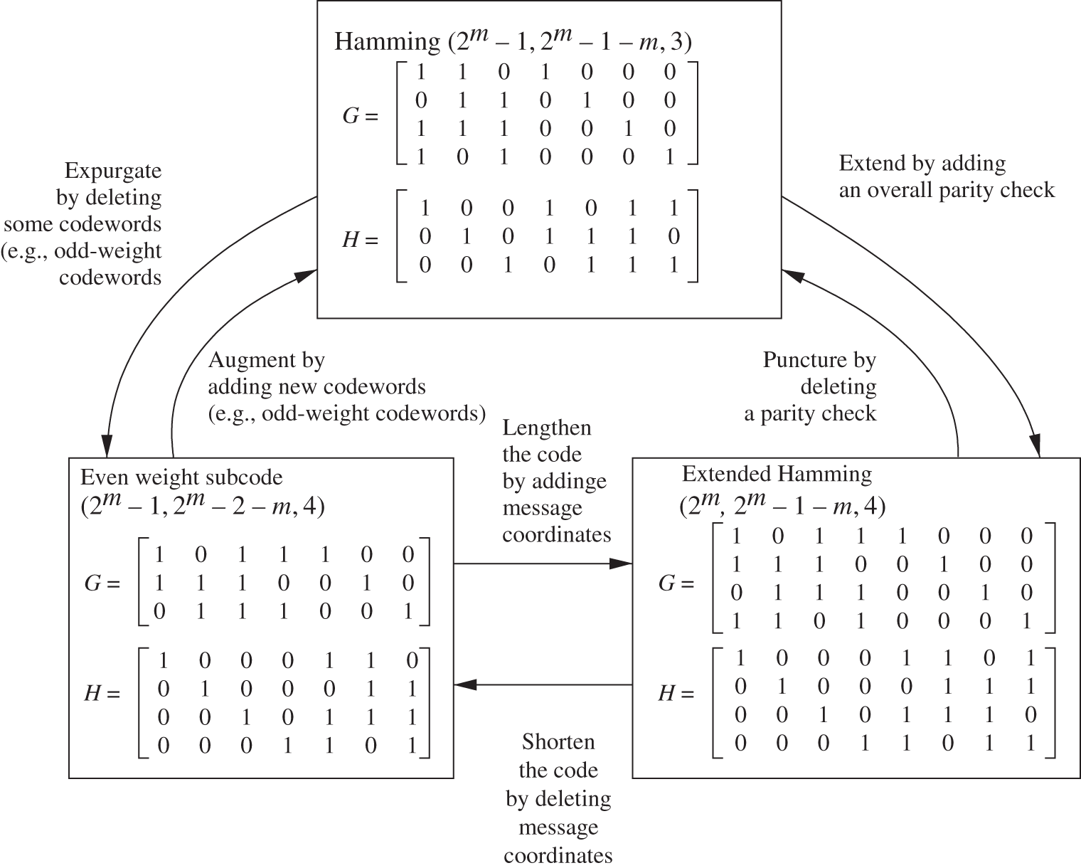
Figure 3.2 Demonstrating modifications on a Hamming code.
Puncturing an extended code can return it to the original code (if the extended symbols are the ones punctured). Puncturing can reduce the weight of each codeword by its weight in the punctured positions. The minimum distance of a code is reduced by puncturing if the minimum weight codeword is punctured in a nonzero position. Puncturing an ![]() code
code ![]() times can result in a code with minimum distance as small as
times can result in a code with minimum distance as small as ![]() .
.
3.10 Best‐Known Linear Block Codes
Tables of the best‐known linear block codes are available. An early version appears in [292]. More recent tables can be found at [50].
Exercises
- 3.1 Find, by trial and error, a set of four binary codewords of length three such that each word is at least a distance of 2 from every other word.
- 3.2 Find a set of 16 binary words of length 7 such that each word is at least a distance of 3 from every other word. Hint: Hamming code.
- 3.3 Perhaps the simplest of all codes is the binary parity check code, a
 code, where
  . Given a message vector
  , the codeword is
  , where
  (arithmetic in
  ) is the parity bit. Such a code is called an even parity code, since all codewords have even parity — an even number of 1 bits.
- Determine the minimum distance for this code.
- How many errors can this code correct? How many errors can this code detect?
- Determine a generator matrix for this code.
- Determine a parity check matrix for this code.
- Suppose that bit errors occur independently with probability
 . The probability that a parity check is satisfied is the probability that an even number of bit errors occur in the received codeword. Verify the following expression for this probability:

- 3.4 For the
 repetition code, determine a parity check matrix.
 - 3.5 [483] Let
 be the probability that any bit in a received vector is incorrect. Compute the probability that the received vector contains undetected errors given the following encoding schemes:
- No code, word length
 .
. - Even parity (see Exercise 3.3 3.3), word length
 .
. - Odd parity, word length
 . (Is this a linear code?)
 - Even parity, word length =
 .
.
- No code, word length
- 3.6 [272] Let
 be an
be an  binary linear systematic code with generator
  . Let
. Let  be an
be an  binary linear systematic code with generator
  . Form the parity check matrix for an
  code as
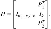
Show that this code has minimum distance at least
 .
. - 3.7 The generator matrix for a code over
 is given by

Find a generator matrix and parity check matrix for an equivalent systematic code.
- 3.8 The generator and parity check matrix for a binary code
 are given by
This code is small enough that it can be used to demonstrate several concepts from throughout the chapter.
- Verify that
 is a parity check matrix for this generator.
 - Draw a logic diagram schematic for an implementation of an encoder for the nonsystematic generator
 using ”and” and ”xor” gates.
 - Draw a logic diagram schematic for an implementation of a circuit that computes the syndrome.
- List the vectors in the orthogonal complement of the code (that is, the vectors in the dual code
 ).
). - Form the standard array for code
 .
. - Form the syndrome decoding table for
 .
. - How many codewords are there of weight
 in
in  ? Determine the weight enumerator
  .
. - Using the generator matrix in (3.23), find the codeword with
 as message bits.
 - Decode the received word
 using the generator of (3.23).
 - Determine the weight enumerator for the dual code.
- Write down an explicit expression for
 for this code. Evaluate this when
  .
. - Write down an explicit expression for
 for this code. Evaluate this when
  .
. - Write down an explicit expression for
 for this code. Evaluate this when
  .
. - Write down an explicit expression for
 for this code, assuming a bounded distance decoder is used. Evaluate this when
  .
. - Write down an explicit expression for
 for this code. Evaluate this when
  .
. - Determine the generator
 for an extended code, in systematic form.
 - Determine the generator for a code which has expurgated all codewords of odd weight. Then express it in systematic form.
- Verify that
- 3.9 [271] Let a binary systematic
 code have parity check equations

- Determine the generator matrix
 for this code in systematic form. Also determine the parity check matrix
  .
. - Using Theorem 3.13, show that the minimum distance of this code is 4.
- Determine
 for this code. Determine
  .
. - Show that this is a self‐dual code.
- Determine the generator matrix
- 3.10 Show that a self‐dual code has a generator matrix
 which satisfies
  .
. - 3.11 Given a code with a parity check matrix
 , show that the coset with syndrome
  contains a vector of weight
  if and only if some linear combination of
  columns of
  equals
  .
. - 3.12 Show that all of the nonzero codewords of the
 simplex code have weight
  . Hint: Start with
  and work by induction.
 - 3.13 Show that (3.13) follows from (3.12).
- 3.14 Show that (3.16) follows from (3.15) using the MacWilliams identity.
- 3.15 Let
 , for
, for  . Determine the Hadamard transform
  of
of  .
. - 3.16 The weight enumerator
 of (3.11) for a code
  is sometimes written as
In this problem, consider binary codes,
 .
.- Show that
 .
. - Let
 be the weight enumerator for the code dual to
  . Show that the MacWilliams identity can be written as
or
- In the following subproblems, assume a binary code. Let
 in (3.24). We can write
Set
 in this and show that
  . Justify this result.
 - Now differentiate (3.25) with respect to
 and set
  to show that

If
 , this gives the average weight.
 - Differentiate (3.25)
 times with respect to
  and set
  to show that
Hint: Define
 . We have the following generalization of the product rule for differentiation:
- Now set
 in (3.24) and write
Differentiate
 times with respect to
  and set
  to show that(3.26)
- Show that
- 3.17 Let
 be a binary
  code with weight enumerator
  and let
  be the extended code of length
  ,
,
Determine the weight enumerator for
 .
. - 3.18 [272] Let
 be a binary linear code with both even‐ and odd‐weight codewords. Show that the number of even‐weight codewords is equal to the number of odd‐weight codewords.
 - 3.19 Show that for a binary code,
 can be written as:

- and
 .
.
- 3.20 [483] Find the lower bound on required redundancy for the following codes.
- A single‐error correcting binary code of length 7.
- A single‐error correcting binary code of length 15.
- A triple‐error correcting binary code of length 23.
- A triple‐error correcting 4‐ary code (i.e.,
 ) of length 23.
- 3.21 Show that all odd‐length binary repetition codes are perfect.
- 3.22 Show that Hamming codes achieve the Hamming bound.
- 3.23 Determine the weight distribution for a binary Hamming code of length 31. Determine the weight distribution of its dual code.
- 3.24 The parity check matrix for a nonbinary Hamming code of length
 and dimension
  with minimum distance 3 can be constructed as follows. For each
  ‐ary
‐ary  ‐tuple of the base‐
 representation of the numbers from 1 to
  , select those for which the first nonzero element is equal to 1. The list of all such
  ‐tuples as columns gives the generator
  .
.
- Explain why this gives the specified length
 .
. - Write down a parity check matrix in systematic form for the
 Hamming code over the field of four elements.
 - Write down the corresponding generator matrix. Note: in this field, every element is its own additive inverse:
 ,
,  ,
,  .
.
- Explain why this gives the specified length
- 3.25 [272] Let
 be the generator matrix of an
  binary code
  and let no column of
  be all zeros. Arrange all the codewords of
  as rows of a
  array.
- Show that no column of the array contains only zeros.
- Show that each column of the array consists of
 zeros and
  ones.
ones. - Show that the set of all codewords with zeros in particular component positions forms a subspace of
 . What is the dimension of this subspace?
 - Show that the minimum distance
 of this code must satisfy the following inequality, known as the Plotkin bound:

- 3.26 [272] Let
 be the ensemble of all the binary systematic linear
  codes.
- Prove that a nonzero binary vector
 is contained in exactly
  of the codes in
  or it is in none of the codes in
  .
. - Using the fact that the nonzero
 ‐tuples of weight
  or less can be in at most
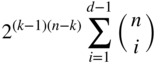
 systematic binary linear codes, show that there exists an
  linear code with minimum distance of at least
  if the following bound is satisfied:
- Show that there exists an
 binary linear code with minimum distance at least
  that satisfies the following inequality:

This provides a lower bound on the minimum distance attainable with an
 linear code known as the Gilbert–Varshamov bound.
- Prove that a nonzero binary vector
- 3.27 Define a linear
 code over
  by the generator matrix

- Find the parity check matrix.
- Prove that this is a single‐error‐correcting code.
- Prove that it is a double‐erasure‐correcting code.
- Prove that it is a perfect code.
- 3.28 [271] Let
 be the parity check matrix for an
  linear code
  . Let
. Let  be the extended code whose parity check matrix
  is formed by

- Show that every codeword of
 has even weight.
 - Show that
 can be obtained from
  by adding an extra parity bit called the overall parity bit to each codeword.
- Show that every codeword of
- 3.29 The
 construction: Let
  ,
,  be linear binary
  block codes with generator matrix
  and minimum distance
  . Define the code
  by
by

- Show that
 has the generator

- Show that the minimum distance of
 is
is

- Show that


3.12 References
The definitions of generator, parity check matrix, distance, and standard arrays are standard; see, for example, [271, 483]. The MacWilliams identity appeared in [291]. Extensions to nonlinear codes appear in [292]. The discussion of probability of error in Section 3.7 is drawn closely from [483]. Our discussion on modifications follows [483], which, in turn, draws from [33]. Our analysis of soft‐input decoding was drawn from [26]. Classes of perfect codes are in [444].
Note
- 1 Most signal processing and communication work employs column vectors by convention. However, a venerable tradition in coding theory has employed row vectors and we adhere to that through most of the book.