CHAPTER 1
Algorithm Basics
Before you jump into the study of algorithms, you need a little background. To begin with, you need to know that, simply stated, an algorithm is a recipe for getting something done. It defines the steps for performing a task in a certain way.
That definition seems simple enough, but no one writes algorithms for performing extremely simple tasks. No one writes instructions for how to access the fourth element in an array. It is just assumed that this is part of the definition of an array and that you know how to do it (if you know how to use the programming language in question).
Normally, people write algorithms only for difficult tasks. Algorithms explain how to find the solution to a complicated algebra problem, how to find the shortest path through a network containing thousands of streets, or how to find the best mix of hundreds of investments to optimize profits.
This chapter explains some of the basic algorithmic concepts you should understand if you want to get the most out of your study of algorithms.
It may be tempting to skip this chapter and jump to studying specific algorithms, but you should at least skim this material. Pay close attention to the section “Big O Notation,” because a good understanding of run time performance can mean the difference between an algorithm performing its task in seconds, hours, or not at all.
Approach
To get the most out of an algorithm, you must be able to do more than simply follow its steps. You need to understand the following:
- The algorithm's behavior Does it find the best possible solution, or does it just find a good solution? Could there be multiple best solutions? Is there a reason to pick one “best” solution over the others?
- The algorithm's speed Is it fast? Slow? Is it usually fast but sometimes slow for certain inputs?
- The algorithm's memory requirements How much memory will the algorithm need? Is this a reasonable amount? Does the algorithm require billions of terabytes more memory than a computer could possibly have (at least today)?
- The main techniques the algorithm uses Can you reuse those techniques to solve similar problems?
This book covers all of these topics. It does not, however, attempt to cover every detail of every algorithm with mathematical precision. It uses an intuitive approach to explain algorithms and their performance, but it does not analyze performance in rigorous detail. Although that kind of proof can be interesting, it can also be confusing and take up a lot of space, providing a level of detail that is unnecessary for most programmers. This book, after all, is intended primarily for programmers who need to get a job done.
This book's chapters group algorithms that have related themes. Sometimes the theme is the task that they perform (sorting, searching, network algorithms), sometimes it's the data structures they use (linked lists, arrays, hash tables, trees), and sometimes it's the techniques they use (recursion, decision trees, distributed algorithms). At a high level, these groupings may seem arbitrary, but when you read about the algorithms, you'll see that they fit together.
In addition to those categories, many algorithms have underlying themes that cross chapter boundaries. For example, tree algorithms (Chapters 10, 11, and 12) tend to be highly recursive (Chapter 15). Linked lists (Chapter 3) can be used to build arrays (Chapter 4), hash tables (Chapter 8), stacks (Chapter 5), and queues (Chapter 5). The ideas of references and pointers are used to build linked lists (Chapter 3), trees (Chapters 10, 11, and 12), and networks (Chapters 13 and 14). As you read, watch for these common threads. Appendix A summarizes common strategies programs use to make these ideas easier to follow.
Algorithms and Data Structures
An algorithm is a recipe for performing a certain task. A data structure is a way of arranging data to make solving a particular problem easier. A data structure could be a way of arranging values in an array, a linked list that connects items in a certain pattern, a tree, a graph, a network, or something even more exotic.
Algorithms are often closely tied to data structures. For example, the edit distance algorithm described in Chapter 15, “String Algorithms,” uses a network to determine how similar two strings are. The algorithm is tied closely to the network and won't work without it. Conversely, the algorithm builds and uses the network, so the network isn't useful (or really even built) without the algorithm.
Often an algorithm says, “Build a certain data structure and then use it in a certain way.” The algorithm can't exist without the data structure, and there's no point in building the data structure if you don't plan to use it with the algorithm.
Pseudocode
To make the algorithms described in this book as useful as possible, they are first described in intuitive English terms. From this high-level explanation, you should be able to implement the algorithm in most programming languages.
Often, however, an algorithm's implementation contains petty details that can make implementation hard. To make handling those details easier, many algorithms are also described in pseudocode. Pseudocode is text that is a lot like a programming language but is not really a programming language. The idea is to give you the structure and details you would need to implement the algorithm in code without tying the algorithm to a particular programming language. Ideally, you can translate the pseudocode into actual code to run on your computer.
The following snippet shows an example of pseudocode for an algorithm that calculates the greatest common divisor (GCD) of two integers:
// Find the greatest common divisor of a and b.
// GCD(a, b) = GCD(b, a Mod b).
Integer: Gcd(Integer: a, Integer: b)
    While (b != 0)
        // Calculate the remainder.
        Integer: remainder = a Mod b

        // Calculate GCD(b, remainder).
        a = b
	b = remainder
    End While

    // GCD(a, 0) is a.
    Return a
End Gcd
The pseudocode starts with a comment. Comments begin with the characters // and extend to the end of the line.
The first actual line of code is the algorithm's declaration. This algorithm is called Gcd and returns an integer result. It takes two parameters named a and b, both of which are integers.
The code after the declaration is indented to show that it is part of the method. The first line in the method's body begins a While loop. The code indented below the While statement is executed as long as the condition in the While statement remains true.
The While loop ends with an End While statement. This statement isn't strictly necessary, because the indentation shows where the loop ends, but it provides a reminder of what kind of block of statements is ending.
The method exits at the Return statement. This algorithm returns a value, so this Return statement indicates which value the algorithm should return. If the algorithm doesn't return any value, such as if its purpose is to arrange values or build a data structure, the Return statement isn't followed by a return value, or the method may have no Return statement.
The code in this example is fairly close to actual programming code. Other examples may contain instructions or values described in English. In those cases, the instructions are enclosed in angle brackets (<>) to indicate that you need to translate the English instructions into program code.
Normally, when a parameter or variable is declared (in the Gcd algorithm, this includes the parameters a and b and the variable remainder), its data type is given before it followed by a colon, as in Integer: remainder. The data type may be omitted for simple integer looping variables, as in For i = 1 To 10.
One other feature that is different from some programming languages is that a pseudocode For loop may include a Step statement indicating the value by which the looping variable is changed after each trip through the loop. A For loop ends with a Next i statement (where i is the looping variable) to remind you which loop is ending.
For example, consider the following pseudocode:
For i = 100 To 0 Step -5
    // Do something…
Next i
This code is equivalent to the following C# code:
for (int i = 100; i >= 0; i -= 5)
{
    // Do something…
}
Both of those are equivalent to the following Python code:
for i in range(100, -1, -5):
    # Do something…
The pseudocode used in this book uses If-Then-Else statements, Case statements, and other statements as needed. These should be familiar to you from your knowledge of real programming languages. Anything else that the code needs is spelled out in English.
Many algorithms in this book are written as methods or functions that return a result. The method's declaration begins with the result's data type. If a method performs some task and doesn't return a result, it has no data type.
The following pseudocode contains two methods:
// Return twice the input value.
Integer: DoubleIt(Integer: value)
    Return 2 * value
End DoubleIt

// The following method does something and doesn't return a value.
DoSomething(Integer: values[])
     // Some code here.
     …
End DoSomething
The DoubleIt method takes an integer as a parameter and returns an integer. The code doubles the input value and returns the result.
The DoSomething method takes as a parameter an array of integers named values. It performs a task and doesn't return a result. For example, it might randomize or sort the items in the array. (Note that this book assumes that arrays start with the index 0. For example, an array containing three items has indices 0, 1, and 2.)
Pseudocode should be intuitive and easy to understand, but if you find something that doesn't make sense to you, feel free to post a question on the book's discussion forum at www.wiley.com/go/essentialalgorithms or e-mail me at [email protected]. I'll point you in the right direction.
One problem with pseudocode is that it has no compiler to detect errors. As a check of the basic algorithm and to give you some actual code to use for a reference, C# and Python implementations of many of the algorithms and exercises are available for download on the book's website.
Algorithm Features
A good algorithm must have three features: correctness, maintainability, and efficiency.
Obviously, if an algorithm doesn't solve the problem for which it was designed, it's not much use. If it doesn't produce correct answers, there's little point in using it.
If an algorithm isn't maintainable, it's dangerous to use in a program. If an algorithm is simple, intuitive, and elegant, you can be confident that it is producing correct results and you can fix it if it doesn't. If the algorithm is intricate, confusing, and convoluted, you may have a lot of trouble implementing it, and you will have even more trouble fixing it if a bug arises. If it's hard to understand, how can you know if it is producing correct results?
Most developers spend a lot of effort on efficiency, and efficiency is certainly important. If an algorithm produces a correct result and is simple to implement and debug, it's still not much use if it takes seven years to finish or if it requires more memory than a computer can possibly hold.
To study an algorithm's performance, computer scientists ask how its performance changes as the size of the problem changes. If you double the number of values the algorithm is processing, does the run time double? Does it increase by a factor of 4? Does it increase exponentially so that it suddenly takes years to finish?
You can ask the same questions about memory usage or any other resource that the algorithm requires. If you double the size of the problem, does the amount of memory required double?
You can also ask the same questions with respect to the algorithm's performance under different circumstances. What is the algorithm's worst-case performance? How likely is the worst case to occur? If you run the algorithm on a large set of random data, what is its average-case performance?
To get a feeling for how problem size relates to performance, computer scientists use Big O notation, which is described in the following section.
Big O Notation
Big O notation uses a function to describe how the algorithm's worst-case performance relates to the problem size as the size grows very large. (This is sometimes called the program's asymptotic performance.) The function is written within parentheses after a capital letter O.
For example, ![]() means that an algorithm's run time (or memory usage or whatever you're measuring) increases as the square of the number of inputs N. If you double the number of inputs, the run time increases by roughly a factor of 4. Similarly, if you triple the number of inputs, the run time increases by a factor of 9.
means that an algorithm's run time (or memory usage or whatever you're measuring) increases as the square of the number of inputs N. If you double the number of inputs, the run time increases by roughly a factor of 4. Similarly, if you triple the number of inputs, the run time increases by a factor of 9.
There are five basic rules for calculating an algorithm's Big O notation.
- If an algorithm performs a certain sequence of steps
 times for a mathematical function f, then it takes
  steps.
 - If an algorithm performs an operation that takes
 steps and then performs a second operation that takes
  steps for functions f and g, then the algorithm's total performance is
  .
. - If an algorithm takes
 time and the function
  is greater than
  for large N, then the algorithm's performance can be simplified to
  .
. - If an algorithm performs an operation that takes
 steps, and for every step in that operation it performs another
  steps, then the algorithm's total performance is
  .
. - Ignore constant multiples. If C is a constant,
 is the same as
  , and
, and  is the same as
  .
.
These rules may seem a bit formal, with all that talk of ![]() and
and ![]() , but they're fairly easy to apply. If they seem confusing, a few examples should make them easier to understand.
, but they're fairly easy to apply. If they seem confusing, a few examples should make them easier to understand.
Rule 1
If an algorithm performs a certain sequence of steps ![]() times for a mathematical function f, then it takes
times for a mathematical function f, then it takes ![]() steps.
steps.
Consider the following algorithm, written in pseudocode, for finding the largest integer in an array:
Integer: FindLargest(Integer: array[])
    Integer: largest = array[0]
    For i = 1 To <largest index>
        If (array[i] > largest) Then largest = array[i]
    Next i
    Return largest
End FindLargest
The FindLargest algorithm takes as a parameter an array of integers and returns an integer result. It starts by setting the variable largest equal to the first value in the array.
It then loops through the remaining values in the array, comparing each to largest. If it finds a value that is larger than largest, the program sets largest equal to that value.
After it finishes the loop, the algorithm returns largest.
This algorithm examines each of the N items in the array once, so it has ![]() performance.
performance.
Rule 2
If an algorithm performs an operation that takes ![]() steps and then performs a second operation that takes
steps and then performs a second operation that takes ![]() steps for functions f and g, then the algorithm's total performance is
steps for functions f and g, then the algorithm's total performance is ![]() .
.
If you look again at the FindLargest algorithm shown in the preceding section, you'll see that a few steps are not actually inside the loop. The following pseudocode shows the same steps, with their run time order shown to the right in comments:
Integer: FindLargest(Integer: array[])
    Integer: largest = array[0]                           // O(1)
    For i = 1 To <largest index>                          // O(N)
        If (array[i] > largest) Then largest = array[i]
    Next i
    Return largest                                        // O(1)
End FindLargest
This algorithm performs one setup step before it enters its loop and then performs one more step after it finishes the loop. Both of those steps have performance O(1) (they're each just a single step), so the total run time for the algorithm is really ![]() . You can use normal algebra to combine terms to rewrite this as
. You can use normal algebra to combine terms to rewrite this as ![]() .
.
Rule 3
If an algorithm takes ![]() time and the function
time and the function ![]() is greater than
is greater than ![]() for large N, then the algorithm's performance can be simplified to
for large N, then the algorithm's performance can be simplified to ![]() .
.
The preceding example showed that the FindLargest algorithm has run time ![]() . When N grows large, the function N is larger than the constant value 2, so
. When N grows large, the function N is larger than the constant value 2, so ![]() simplifies to
simplifies to ![]() .
.
Ignoring the smaller function lets you focus on the algorithm's asymptotic behavior as the problem size becomes very large. It also lets you ignore relatively small setup and cleanup tasks. If an algorithm spends some time building simple data structures and otherwise getting ready to perform a big computation, you can ignore the setup time as long as it's small compared to the length of the main calculation.
Rule 4
If an algorithm performs an operation that takes ![]() steps, and for every step in that operation it performs another
steps, and for every step in that operation it performs another ![]() steps, then the algorithm's total performance is
steps, then the algorithm's total performance is ![]() .
.
Consider the following algorithm that determines whether an array contains any duplicate items. (Note that this isn't the most efficient way to detect duplicates.)
Boolean: ContainsDuplicates(Integer: array[])
    // Loop over all of the array's items.
    For i = 0 To <largest index>
        For j = 0 To <largest index>
            // See if these two items are duplicates.
	    If (i != j) Then
                If (array[i] == array[j]) Then Return True
            End If
        Next j
    Next i
    // If we get to this point, there are no duplicates.
    Return False
End ContainsDuplicates
This algorithm contains two nested loops. The outer loop iterates over all the array's N items, so it takes ![]() steps.
steps.
For each trip through the outer loop, the inner loop also iterates over the N items in the array, so it also takes ![]() steps.
steps.
Because one loop is nested inside the other, the combined performance is ![]() .
.
Rule 5
Ignore constant multiples. If C is a constant, ![]() is the same as
is the same as ![]() , and
, and ![]() is the same as
is the same as ![]() .
.
If you look again at the ContainsDuplicates algorithm shown in the preceding section, you'll see that the inner loop actually performs one or two steps. It performs an If test to see if the indices i and j are the same. If they are different, it compares array[i] and array[j]. It may also return the value True.
If you ignore the extra step for the Return statement (it happens at most only once) and you assume that the algorithm performs both of the If statements (as it does most of the time), then the inner loop takes ![]() steps. Therefore, the algorithm's total performance is
steps. Therefore, the algorithm's total performance is ![]() .
.
Rule 5 lets you ignore the factor of 2, so the run time is ![]() .
.
This rule really goes back to the purpose of Big O notation. The idea is to get a feeling for the algorithm's behavior as N increases. In this case, suppose that you increase N by a factor of 2.
If you plug the value ![]() into the equation
into the equation ![]() , you get the following:
, you get the following:
This is four times the original value ![]() , so the run time has increased by a factor of 4.
, so the run time has increased by a factor of 4.
Now try the same thing with the run time simplified by rule 5 to ![]() . Plugging
. Plugging ![]() into this equation gives the following:
into this equation gives the following:
This is four times the original value ![]() , so this also means that the run time has increased by a factor of 4.
, so this also means that the run time has increased by a factor of 4.
Whether you use the formula ![]() or just
or just ![]() , the result is the same: increasing the size of the problem by a factor of 2 increases the run time by a factor of 4. The important thing here isn't the constant; it's the fact that the run time increases as the square of the number of inputs N.
, the result is the same: increasing the size of the problem by a factor of 2 increases the run time by a factor of 4. The important thing here isn't the constant; it's the fact that the run time increases as the square of the number of inputs N.
Common Run Time Functions
When you study the run time of algorithms, some functions occur frequently. The following sections give some examples of a few of the most common functions. They also give you some perspective so that you'll know, for example, whether an algorithm with ![]() performance is reasonable.
performance is reasonable.
1
An algorithm with O(1) performance takes a constant amount of time no matter how big the problem is. These sorts of algorithms tend to perform relatively trivial tasks because they cannot even look at all of the inputs in O(1) time.
For example, at one point the quicksort algorithm needs to pick a number that is in an array of values. Ideally, that number should be somewhere in the middle of all of the values in the array, but there's no easy way to tell which number might fall nicely in the middle. (For example, if the numbers are evenly distributed between 1 and 100, 50 would make a good dividing number.) The following algorithm shows one common approach for solving this problem:
Integer: DividingPoint(Integer: array[])
    Integer: number1 = array[0]
    Integer: number2 = array[<last index of array>]
    Integer: number3 = array[<last index of array> / 2]

    If (<number1 is between number2 and number3>) Then Return number1
    If (<number2 is between number1 and number3>) Then Return number2
    Return number3
End MiddleValue
This algorithm picks the values at the beginning, end, and middle of the array; compares them; and returns whichever item lies between the other two. This may not be the best item to pick out of the whole array, but there's a decent chance that it's not too terrible a choice.
Because this algorithm performs only a few fixed steps, it has O(1) performance and its run time is independent of the number of inputs N. (Of course, this algorithm doesn't really stand alone. It's just a small part of a more complicated algorithm.)
Log N
An algorithm with ![]() performance typically divides the number of items it must consider by a fixed fraction at every step.
performance typically divides the number of items it must consider by a fixed fraction at every step.
For example, Figure 1.1 shows a sorted complete binary tree. It's a binary tree because every node has at most two branches. It's a complete tree because every level (except possibly the last) is completely full, and all the nodes in the last level are grouped on the left side. It's a sorted tree because every node's value is at least as large as its left child and no larger than its right child. (Chapter 10, “Trees,” has a lot more to say about trees.)
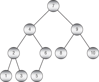
Figure 1.1: Searching a full binary tree takes O(log N) steps.
The following pseudocode shows one way you might search the tree shown in Figure 1.1 to find a particular item:
Node: FindItem(Integer: target_value)
    Node: test_node = <root of tree>

    Do Forever
     // If we fell off the tree. The value isn't present.
     If (test_node == null) Then Return null

     If (target_value == test_node.Value) Then
         // test_node holds the target value.
	 // This is the node we want.
	 Return test_node
     Else If (target_value < test_node.Value) Then
         // Move to the left child.
         test_node = test_node.LeftChild
     Else
         // Move to the right child.
	 test_node = test_node.RightChild
     End If
   End Do
End FindItem
Chapter 10, “Trees,” covers tree algorithms in detail, but you should be able to get the gist of the algorithm from the following discussion.
The algorithm declares and initializes the variable test_node so that it points to the root at the top of the tree. (Traditionally, trees in computer programs are drawn with the root at the top, unlike real trees.) It then enters an infinite loop.
If test_node is null, then the target value isn't in the tree, so the algorithm returns null.
If test_node holds the target value, then test_node is the node that you're seeking, so the algorithm returns it.
If target_value is less than the value in test_node, then the algorithm sets test_node equal to its left child. (If test_node is at the bottom of the tree, its LeftChild value is null, and the algorithm handles the situation the next time it goes through the loop.)
If test_node's value does not equal target_value and is not less than target_value, then it must be greater than target_value. In that case, the algorithm sets test_node equal to its right child. (Again, if test_node is at the bottom of the tree, its RightChild is null, and the algorithm handles the situation the next time it goes through the loop.)
The variable test_node moves down through the tree and eventually either finds the target value or falls off the tree when test_node is null.
Understanding this algorithm's performance becomes a question of how far down the tree test_node must move before it either finds target_value or it falls off the tree.
Sometimes the algorithm gets lucky and finds the target value right away. If the target value is 7 in Figure 1.1, the algorithm finds it in one step and stops. Even if the target value isn't at the root node—for example, if it's 4—the program might have to check only a small piece of the tree before stopping.
In the worst case, however, the algorithm needs to search the tree from top to bottom.
In fact, roughly half the tree's nodes are the nodes at the bottom that have missing children. If the tree were a full complete tree, with every node having exactly zero or two children, then the bottom level would hold exactly half the tree's nodes. That means if you search for randomly chosen values in the tree, the algorithm will have to travel through most of the tree's height most of the time.
Now the question is, “How tall is the tree?” A full complete binary tree of height H has ![]() nodes. To look at it from the other direction, a full complete binary tree that contains N nodes has height
nodes. To look at it from the other direction, a full complete binary tree that contains N nodes has height ![]() . Because the algorithm searches the tree from top to bottom in the worst (and average) case and because the tree has a height of roughly
. Because the algorithm searches the tree from top to bottom in the worst (and average) case and because the tree has a height of roughly ![]() , the algorithm runs in
, the algorithm runs in ![]() time.
time.
At this point, a curious feature of logarithms comes into play. You can convert a logarithm from base A to base B using this formula:
Setting ![]() , you can use this formula to convert the value
, you can use this formula to convert the value ![]() into any other log base A:
into any other log base A:
The value ![]() is a constant for any given A, and Big O notation ignores constant multiples, so that means
is a constant for any given A, and Big O notation ignores constant multiples, so that means ![]() is the same as
is the same as ![]() for any log base A. For that reason, this run time is often written
for any log base A. For that reason, this run time is often written ![]() with no indication of the base (and no parentheses to make it look less cluttered).
with no indication of the base (and no parentheses to make it look less cluttered).
This algorithm is typical of many algorithms that have ![]() performance. At each step, it divides the number of items that it must consider into two, roughly equal-sized groups.
performance. At each step, it divides the number of items that it must consider into two, roughly equal-sized groups.
Because the log base doesn't matter in Big O notation, it doesn't matter which fraction the algorithm uses to divide the items that it is considering. This example divides the number of items in half at each step, which is common for many logarithmic algorithms. But it would still have ![]() performance if it divided the remaining items by a factor of 1/10th and made lots of progress at each step or if it divided the items by a factor of 9/10ths and made relatively little progress.
performance if it divided the remaining items by a factor of 1/10th and made lots of progress at each step or if it divided the items by a factor of 9/10ths and made relatively little progress.
The logarithmic function ![]() grows relatively slowly as N increases, so algorithms with
grows relatively slowly as N increases, so algorithms with ![]() performance generally are fast enough to be useful.
performance generally are fast enough to be useful.
Sqrt N
Some algorithms have ![]() performance (where sqrt is the square root function), but they're not common, and they are not covered in this book. This function grows very slowly but a bit faster than
performance (where sqrt is the square root function), but they're not common, and they are not covered in this book. This function grows very slowly but a bit faster than ![]() .
.
N
The FindLargest algorithm described in the earlier section “Rule 1” has ![]() performance. See that section for an explanation of why it has
performance. See that section for an explanation of why it has ![]() performance.
performance.
The function N grows more quickly than ![]() and
and ![]() but still not very quickly, so most algorithms that have
but still not very quickly, so most algorithms that have ![]() performance work quite well in practice.
performance work quite well in practice.
N log N
Suppose an algorithm loops over all of the items in its problem set and then, for each loop, performs some sort of ![]() calculation on that item. In that case, the algorithm has
calculation on that item. In that case, the algorithm has ![]() or
or ![]() performance.
performance.
Alternatively, an algorithm might perform some sort of ![]() operation and, for each step in it, do something to each of the items in the problem.
operation and, for each step in it, do something to each of the items in the problem.
For example, suppose that you have built a sorted tree containing N items as described earlier. You also have an array of N values and you want to know which values in the array are also in the tree.
One approach would be to loop through the values in the array. For each value, you could use the method described earlier to search the tree for that value. The algorithm examines N items, and for each it performs ![]() steps so the total run time is
steps so the total run time is ![]() .
.
Many sorting algorithms that work by comparing items to each other have an ![]() run time. In fact, it can be proven that any algorithm that sorts by comparing items must use at least
run time. In fact, it can be proven that any algorithm that sorts by comparing items must use at least ![]() steps, so this is the best you can do, at least in Big O notation. Some of those algorithms are still faster than others because of the constants that Big O notation ignores. Some algorithms that don't use comparisons can sort even more quickly. Chapter 6 talks more about algorithms with various run times.
steps, so this is the best you can do, at least in Big O notation. Some of those algorithms are still faster than others because of the constants that Big O notation ignores. Some algorithms that don't use comparisons can sort even more quickly. Chapter 6 talks more about algorithms with various run times.
N2
An algorithm that loops over all of its inputs and then for each input loops over the inputs again has ![]() performance. For example, the
performance. For example, the ContainsDuplicates algorithm described earlier in the section “Rule 4” runs in ![]() time. See that section for a description and analysis of the algorithm.
time. See that section for a description and analysis of the algorithm.
Other powers of N, such as ![]() and
and ![]() , are possible and are obviously slower than
, are possible and are obviously slower than ![]() .
.
An algorithm is said to have polynomial run time if its run time involves any polynomial involving N. ![]() ,
, ![]() ,
, ![]() , and even
, and even ![]() are all polynomial run times.
are all polynomial run times.
Polynomial run times are important because in some sense these problems can still be solved. The exponential and factorial run times described next grow extremely quickly, so algorithms that have those run times are practical for only very small numbers of inputs.
Exponential functions such as ![]() grow extremely quickly, so they are practical for only small problems. Typically algorithms with these run times look for optimal selections of the inputs.
grow extremely quickly, so they are practical for only small problems. Typically algorithms with these run times look for optimal selections of the inputs.
For example, in the knapsack problem, you are given a set of objects that each has a weight and a value. You also have a knapsack that can hold a certain amount of weight. You can put a few heavy items in the knapsack, or you can put lots of lighter items in it. The challenge is to select the items with the greatest total value that fit in the knapsack.
This may seem like an easy problem, but the only known algorithms for finding the best possible solution essentially require you to examine every possible combination of items.
To see how many combinations are possible, note that each item is either in the knapsack or out of it, so each item has two possibilities. If you multiply the number of possibilities for the items, you get ![]() total possible selections.
total possible selections.
Sometimes, you don't have to try every possible combination. For example, if adding the first item fills the knapsack completely, you don't need to add any selections that include the first item plus another item. In general, however, you cannot exclude enough possibilities to narrow the search significantly.
For problems with exponential run times, you often need to use heuristics—algorithms that usually produce good results but that you cannot guarantee will produce the best possible results.
N!
The factorial function, written N! and pronounced “N factorial,” is defined for integers greater than 0 by ![]() . This function grows much more quickly than even the exponential function
. This function grows much more quickly than even the exponential function ![]() . Typically, algorithms with factorial run times look for an optimal arrangement of the inputs.
. Typically, algorithms with factorial run times look for an optimal arrangement of the inputs.
For example, in the traveling salesman problem (TSP), you are given a list of cities. The goal is to find a route that visits every city exactly once and returns to the starting point while minimizing the total distance traveled.
This isn't too hard with just a few cities, but with many cities the problem becomes challenging. The most obvious approach is to try every possible arrangement of cities. Following that algorithm, you can pick N possible cities for the first city. After making that selection, you have ![]() possible cities to visit next. Then there are
possible cities to visit next. Then there are ![]() possible third cities, and so forth, so the total number of arrangements is
possible third cities, and so forth, so the total number of arrangements is ![]() .
.
Visualizing Functions
Table 1.1 shows a few values for the run time functions described in the preceding sections so that you can see how quickly these functions grow.
Table 1.1: Function Values for Various Inputs
| N | log2(N) | sqrt(N) | N | N2 | 2N | N! |
| 1 | 0.00 | 1.00 | 1 | 1.00 | 2 | 1 |
| 5 | 2.32 | 2.23 | 5 | 25 | 32 | 625 |
| 10 | 3.32 | 3.16 | 10 | 100 | 1,024 |
|
| 15 | 3.90 | 3.87 | 15 | 225 |
|
|
| 20 | 4.32 | 4.47 | 20 | 400 |
|
|
| 50 | 5.64 | 7.07 | 50 | 2,500 |
|
|
| 100 | 6.64 | 10.00 | 100 |
|
|
|
| 1000 | 9.96 | 31.62 | 1,000 |
|
|
— |
| 10000 | 13.28 | 100.00 |
|
|
— | — |
| 100000 | 16.60 | 316.22 |
|
|
— | — |
Figure 1.2 shows a graph of these functions. Some of the functions have been scaled so that they fit better on the graph, but you can easily see which grows fastest when x grows large. Even dividing by 100 doesn't keep the factorial function on the graph for very long.
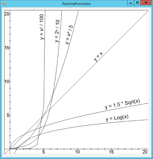
Figure 1.2: The log, sqrt, linear, and even polynomial functions grow at a reasonable pace, but exponential and factorial functions grow incredibly quickly.
Practical Considerations
Although theoretical behavior is important in understanding an algorithm's run time behavior, practical considerations also play an important role in real-world performance for several reasons.
The analysis of an algorithm typically considers all steps as taking the same amount of time even though that may not be the case. Creating and destroying new objects, for example, may take much longer than moving integer values from one part of an array to another. In that case, an algorithm that uses arrays may outperform one that uses lots of objects even though the second algorithm does better in Big O notation.
Many programming environments also provide access to operating system functions that are more efficient than basic algorithmic techniques. For example, part of the insertionsort algorithm requires you to move some of the items in an array down one position so that you can insert a new item before them. This is a fairly slow process and contributes greatly to the algorithm's ![]() performance. However, many programs can use a function (such as
performance. However, many programs can use a function (such as RtlMoveMemory in .NET programs and MoveMemory in Windows C++ programs) that moves blocks of memory all at once. Instead of walking through the array, moving items one at a time, a program can call these functions to move the whole set of array values at once, making the program much faster.
Just because an algorithm has a certain theoretical asymptotic performance doesn't mean that you can't take advantage of whatever tools your programming environment offers to improve performance. Some programming environments also provide tools that can perform the same tasks as some of the algorithms described in this book. For example, many libraries include sorting routines that do a very good job of sorting arrays. Microsoft's .NET Framework, used by C# and Visual Basic, includes an Array.Sort method that uses an implementation that you are unlikely to beat using your own code—at least in general. Similarly, Python lists have a sort method that sorts the items in the list.
For specific problems, you can still sometimes beat built-in sorting methods if you have extra information about the data. (For example, read about countingsort in Chapter 6.)
Special-purpose libraries may also be available that can help you with certain tasks. For example, you may be able to use a network analysis library instead of writing your own network tools. Similarly, database tools may save you a lot of work building trees and sorting things. You may get better performance building your own balanced trees, but using a database is a lot less work.
If your programming tools include functions that perform the tasks of one of these algorithms, by all means use them. You may get better performance than you could achieve on your own, and you'll certainly have less debugging to do.
Finally, the best algorithm isn't always the one that is fastest for very large problems. If you're sorting a huge list of numbers, quicksort usually provides good performance. If you're sorting only three numbers, a simple series of If statements will probably give better performance and will be a lot simpler. Even if quicksort does give better performance, does it matter whether the program finishes sorting in 1 millisecond or 2? Unless you plan to perform the sort many times, you may be better off going with the simpler algorithm that's easier to debug and maintain rather than the complicated one to save 1 millisecond.
If you use libraries such as those described in the preceding paragraphs, you may not need to code all of these algorithms yourself, but it's still useful to understand how the algorithms work. If you understand the algorithms, you can take better advantage of the tools that implement them even if you don't write them. For example, if you know that relational databases typically use B-trees (and similar trees) to store their indices, you'll have a better understanding of how important pre-allocation and fill factors are. If you understand quicksort, you'll know why some people think the .NET Framework's Array.Sort method is not cryptographically secure. (This is discussed in the section “Using Quicksort” in Chapter 6.)
Understanding the algorithms also lets you apply them to other situations. You may not need to use mergesort, but you may be able to use its divide-and-conquer approach to solve some other problem on multiple processors.
Summary
To get the most out of an algorithm, you not only need to understand how it works, but you also need to understand its performance characteristics. This chapter explained Big O notation, which you can use to study an algorithm's performance. If you know an algorithm's Big O run time behavior, you can estimate how much the run time will change if you change the problem size.
This chapter also described some algorithmic situations that lead to common run time functions. Figure 1.2 showed graphs of these equations so that you can get a feel for just how quickly each grows as the problem size increases. As a rule of thumb, algorithms that run in polynomial time are often fast enough that you can run them for moderately large problems. Algorithms with exponential or factorial run times, however, grow extremely quickly as the problem size increases, so you can run them only with relatively small problem sizes.
Now that you have some understanding of how to analyze algorithm speeds, you're ready to study some specific algorithms. The next chapter discusses numerical algorithms. They tend not to require elaborate data structures, so they usually are quite fast.
Exercises
You can find the answers to these exercises in Appendix B. Asterisks indicate particularly difficult problems.
- The section “Rule 4” described a
ContainsDuplicatesalgorithm that has run time . Consider the following improved version of that algorithm:
Boolean: ContainsDuplicates(Integer: array[])
    // Loop over all of the array's items except the last one.
    For i = 0 To <largest index> - 1
        // Loop over the items after item i.
	For j = i + 1 To <largest index>
            // See if these two items are duplicates.
	    If (array[i] == array[j]) Then Return True
        Next j
    Next i

    // If we get to this point, there are no duplicates.
    Return False
End ContainsDuplicates
What is the run time of this new version?
- Table 1.1 showed the relationship between problem size N and various run time functions. Another way to study that relationship is to look at the largest problem size that a computer with a certain speed could execute within a given amount of time.
For example, suppose a computer can execute 1 million algorithm steps per second. Consider an algorithm that runs in
 time. In one hour, the computer could solve a problem where
  (because
  which is the number of steps the computer can execute in one hour).
Make a table showing the largest problem size N that this computer could execute for each of the functions listed in Table 1.1 in one second, minute, hour, day, week, and year.
- Sometimes the constants that you ignore in Big O notation are important. For example, suppose that you have two algorithms that can do the same job. The first requires
 steps, and the other requires
  steps. For what values of N would you choose each algorithm?
 - *Suppose you have two algorithms—one that uses
 steps, and one that uses
  steps. For what values of N would you choose each algorithm?
 - Suppose a program takes as inputs N letters and generates all possible unordered pairs of the letters. For example, with inputs ABCD, the program generates the combinations AB, AC, AD, BC, BD, and CD. (Here unordered means that AB and BA count as the same pair.) What is the algorithm's run time?
- Suppose an algorithm with N inputs generates values for each unit square on the surface of an
 cube. What is the algorithm's run time?
 - Suppose an algorithm with N inputs generates values for each unit cube on the edges of an
 cube, as shown in Figure 1.3. What is the algorithm's run time?
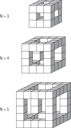
Figure 1.3: This algorithm generates values for cubes on a cube's “skeleton.” - *Suppose you have an algorithm that, for N inputs, generates a value for each small cube in the shapes shown in Figure 1.4. Assuming that the obvious hidden cubes are present so that the shapes in the figure are not hollow, what is the algorithm's run time?
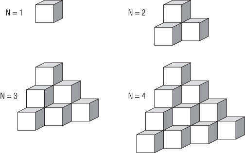
Figure 1.4: This algorithm adds one more level to the shape as N increases. - Can you have an algorithm without a data structure? Can you have a data structure without an algorithm?
- Consider the following two algorithms for painting a fence:
Algorithm1()
    For i = 0 To <number of boards in fence> - 1
        <paint board number i>
    Next i
End Algorithm1

Algorithm2(Integer: first_board, Integer: last_board)
    If (first_board == last_board) Then
        // There's only one board. Just paint it.
	<paint board number first_board>
    Else
       // There's more than one board. Divide the boards
       // into two groups and recursively paint them.
       Integer: middle_board = (first_board + last_board) / 2
       Algorithm2(first_board, middle_board)
       Algorithm2(middle_board + 1, last_board)
    End If
End Algorithm2
What are the run times for these two algorithms, where N is the number of boards in the fence? Which algorithm is better?
- *You can define Fibonacci numbers recursively by the following rules:
Fibonacci(0) = 1
Fibonacci(1) = 1
Fibonacci(n) = Fibonacci(n - 1) + Fibonacci(n - 2)
The Fibonacci sequence starts with the values 1, 1, 2, 3, 5, 8, 13, 21, 34, 55, 89.
How does the Fibonacci function compare to the run time functions shown in Figure 1.2?