Chapter 2. Probability
When you think of probability, what images come to mind? Perhaps you think of gambling-related examples, like the probability of winning the lottery or getting a pair with two dice. Maybe it is predicting stock performance, the outcome of a political election, or whether your flight will arrive on time. Our world is full of uncertainties we want to measure.
Maybe that is the word we should focus on: uncertainty. How do we measure something that we are uncertain about? This is an interesting question that has created two schools of thought: Frequentism and Bayesianism. It is also a source of anxiety for many technical professionals used to deterministic and predictable outcomes. For example, software engineers have a “unit test” mindset where software executes with absolute logic that predictably runs the same way every time. However models that output approximations of random events are a very different animal.
In the end, probability is about measuring our certainty (or uncertainty) that an event will happen. It is a foundational discipline for statistics, hypothesis testing, machine learning, and other topics in this book. A lot of folks take probability for granted and assume they understand it. However, it is more nuanced and complicated than most people think. While the theorems and ideas of probability are mathematically sound, it gets more complex when we introduce data and venture into statistics. We will cover that in Chapter 4 on statistics and hypothesis testing.
In this chapter, we will discuss what probability is. Then we will cover probability math concepts, Bayes Theorem, the Binomial Distribution, and the Beta Distribution.
Understanding Probability
Probability is how strongly we believe, based on observations or belief, an event will happen often expressed as a proportion. Here are some questions that might warrant a probability for an answer:
-
How likely will I get 7 heads in 10 fair coin flips?
-
What are my chances in winning an election?
-
Will my flight be late?
-
How certain am I a product is defective?
The most popular way to express probability is as a percentage, as in “There is a 70% chance my flight will be late.” We will call this probability P(X), where X is the event of interest. As you work with probabilities though, you will more likely see it expressed as a decimal (in this case .70) which must be between 0.0 and 1.0.
Likelihood is similar to probability, and it is easy to confuse the two ( many dictionaries and even statisticians do as well). You can even get away with using “probability” and “likelihood” interchangeably in everyday conversation. However, we should pin down these differences. Probability is about quantifying predictions of events yet to happen, whereas likelihood is measuring the frequency of events that already occurred. In statistics and machine learning, we often use likelihood (the past) to predict probability (the future).
It is important to note that a probability of an event happening must be strictly between 0% and 100%, or 0.0 and 1.0. Logically, this means the probability of an event NOT happening is calculated by subtracting the probability of the event from 1.0.
Alternatively, probability can be expressed as an odds ratio
While many people feel more comfortable expressing probabilities as percentages or proportions, odds ratios can be a helpful tool. If I have an odds ratio of 2.0, that means I feel an event is 2 times more likely to happen than not to happen. That can be more intuitive to describe a belief than a percentage of
To turn an odds ratio
So if have an odds ratio
Conversely, you can turn an odds ratio into a probability simply by dividing the probability of the event occuring by the probability it will not occur:
Probability versus Statistics
Sometimes people use the terms probability and statistics interchangeably, and while this is understandable to conflate the two disciplines they do have distinctions. Probability is the study of how likely an event is to happen. Statistics utilizes data to discover probability and provides tools to decribe data. You can have probability without statistics, but statistics is pretty limited without probability.
Think of predicting the outcome of rolling a “4” on a die (that’s the singular of “dice”). Approaching the problem with a pure probability mindset, one simply says there are 6 sides on a die. We assume each side is equally likely, so the probability of getting a “4” is
However, a zealous statistician might say “No! We need to roll the die to get data. If we can get 30 rolls or more, and the more rolls we do the better, only then will we have data to determine the probability of getting a 4.” This approach may seem silly if we assume the die is fair, but what if it’s not? If that’s the case, collecting data is the only way to discover the probability of rolling a “4”. We will talk about hypothesis testing in the next chapter.
Frequentist versus Bayesian Probability
While we are discussing statistics’ relationship to probability, let’s talk about two schools of thought on how we use probability. Let’s dissect this statement: “There is a 60% chance my flight will be late.” What exactly does that mean? Stop and think about that for a moment. Where could that “60%” number have come from?
One school of thought will say “Well out of 100 flights in the past similar to this one, 60 of them were late.” This is what we call a Frequentism mindset, where we derive probabilities off historical data and count the frequency of an event. This is a somewhat simplistic definition as I would use confidence intervals and other tools, but that is the essence of Frequentism.
But here comes the Bayesian who says differently. Bayesianism measures probability based on belief. She says “well given the poor weather forecast, a rival college game happening tonight, and the fact a terminal is closed for construction all causing congestion, my gut feel says there is an 80% chance this flight will be late.”
“Wait! You can’t just make up numbers on your gut feel!” says the Frequentist.
The Bayesian retorts “Why not? I fly frequently and have seen bad weather, college games, and terminal construction congest airports and make flights late.”
“Data is truth! And the data says 60% of flights at this time of day are late!”
“I don’t doubt that. As a matter of fact I started my belief with that 60% number as my baseline. I then accounted for the bad weather, the college game, and terminal construction and therefore increased my belief to 80%”
“I still don’t like you made up numbers you never measured” says the Frequentist. “Your conclusions are anecdotal at best!”
So who is right here? Is it the Frequentist or the Bayesian? Before reading on, think about this carefully and what side you should take.
Is it possible both the Frequentist and Bayesian are correct? Absolutely! Consider that Frequentism and Bayesianism both have merits depending on the situation. Frequentism works best when there is enough high quality, consistent data you can reliably draw conclusions from. But when you lack data, the data is unreliable, the data is always changing, or there are just too many chaotic variables you cannot control, Bayesianism can be a great tool to account for uncertainty. You can even merge data and beliefs together to get the best of both worlds.
Even when you do have lots of data, Bayesianism can still be a helpful tool to entertain a span of possibilities. We will see this in action with the Beta distribution where we estimate parameters as distributions rather than a single value.
Regarding the Frequentist accusing the Bayesian of being anecdotal, that is certainly a bias to watch out for. While her experiences should not be generalized for everyone else, she did establish herself as an “expert” because she frequently flies. Bayesianism realizes that beliefs can be just as important in probability, as we may not always have sufficient data on hand and our “experts” and “common sense” are the best tools we have.
We will explore a few more Bayesian ideas in this chapter, and we will talk about statistics and hypothesis testing in Chapter 4.
Probability Math
When we work with a single probability of an event P(X), known as a marginal probability, the idea is fairly straightforward as we discussed previously. But when we start combining probabilities of different events together, it gets a little less intuitive.
Joint Probabilities
Let’s say you have a fair coin and a fair 6-sided die. You want to find the probability of flipping a “Heads” and rolling a “6” on the coin and die respectively. These are two separate probabilities of two separate events, but we want to find the probability that both events will occur together. This is known as a joint probability.
Think of a joint probability as an AND operator. I “want to find the probability of flipping a heads AND rolling a 6.” We want both events to happen together, so how do we calculate this probability?
There are 2 sides on a coin and 6 sides on the die, so the probability of heads is
Easy enough, but why is this the case? A lot of probability rules can be discovered by generating all possible combinations of events, which comes from an area of math known as permutations and combinations. For this case, generate every possible outcome between the coin and die, pairing heads (H) and tails (T) with the numbers 1 through 6:
H1 H2 H3 H4 H5 *H6* T1 T2 T3 T4 T5 T6
Notice there are 12 possible outcomes when flipping our coin and rolling our die. The only one that is of interest to us is “H6,” getting a heads and a six. So because there is only 1 outcome that satisfies our condition, and there are 12 possible outcomes, the probability of getting a heads and a six is
Rather than generate all possible combinations and counting the ones of interest to us, we can use multiplication as a shortcut to find the joint probability. This is known as the product rule.
But what if we are interested in 3 joint events? 10 events? 1000 events? Does the product rule still apply? Yes it does! We just multiply the probability of each event together to find the probability of all events of interest occurring.
If I roll a die three times, what is the probability P(X) of getting a “1” on the first role? A “2” or “4” on the second roll? And a “3”, “4”, or “6” on the third roll?
So the probability of getting that outcome for those 3 rolls is
Floating Point Underflow
— Note to self, move this to later chapter based on reviewer feedback
A problem you can come across when doing joint probabilities on computers is something called floating point underflow, which happens when you multiply a lot of small decimals together. Computers can only keep track of so many decimal places, so when the decimals start getting small your computer gives up and just lets your decimals approach 0. A clever hack you can do (as presented in Joel Grus’ book Data Science from Scratch by O’Reilly) is to take the log() of each probability, add them together, and then call exp() to convert the result back!
In Example 2-1 we use logarithmic addition of probabilities (rather than multiplication) to calculate the probability of 3 consecutive engine failures if probability of each failure is 10%. It really does not matter what base you use for the logarithm, so we can just use the default Euler’s number e.
Example 2-1. Using logarithmic addition to perform joint probabilities
from math import log, exp

prob_engine_failure = .10
three_fails_prob = 0.0

for i in range(0,3):
    # Perform logarithmic addition instead of multiplication
    three_fails_prob += log(prob_engine_failure)

# Use exp() to convert back!
three_fails_prob = exp(three_fails_prob)

# 0.0010000000000000002
print("Probability of 3 consecutive failures: {}".format(three_fails_prob))
Union Probabilities
We discussed joint probabilities, which is the probability of two or more events occurring simultaneously. But what about the probability of getting event A or B? When we deal with “OR” operations with probabilities, this is known as a union probability.
Let’s start with mutually exclusive events, which are events that cannot occur simultaneously. For example, if I roll a die I cannot simultaneously get a “4” and a “6”. I can only get one outcome. Getting the union probability for these cases are easy. I just simply add them together. So if I want to find the probability of getting a “4” or “6” on a die roll:
Just like the joint operation, the union operation extends to more than two events. The probability of getting a “2”, “4” or “6” on a single die roll is
But what about non-mutally exclusive events, which are events that can occur simulataneously? Let’s go back to the coin flip and die roll example. What is the probability of getting a heads OR a “6”? Before you are tempted to add those probabilities, let’s generate all possible outcomes again and highlight the ones we are interested in:
*H1* *H2* *H3* *H4* *H5* *H6* T1 T2 T3 T4 T5 *T6*
Above we are interested in all the “heads” outcome as well as the “6” outcomes. If we proportion the 7 out of 12 outcomes we are interested in,
But what happens if we add the two probabilities of heads and “6” together? We get a different (and wrong!) answer of
Why is that? Study the combinations of coin flip and die outcomes again and see if you can find something fishy. Notice when we add the probabilities, we double-count the probability of getting a “6” for “H6” and “T6”! If this is not clear, try finding the probability of getting “Heads” and a die roll of 1 through 5.
We get a probability of 133.333% which is definitely not correct, as a probability must be no more than 100% or 1.0. The problem again is we are double-counting outcomes.
If you ponder long enough, you may realize the logical way to remove double-counting in a union probability is to subract the joint probability. This is known as the sum rule of probability and ensures every joint event is only counted once.
So going back to our example of calculating the probability of a Heads or a “6”, we need to subtact the joint probability of getting a Heads or a “6” from the union probability:
Note that this formula
In summary, when you have a union probability between two or more events that are not mutually exclusive, be sure to subtract the joint probability so no probabilities are double-counted.
Conditional Probability and Bayes Theorem
A probability topic that people easily get confused by is the concept of conditional probability, which is the probability of an event A occuring given event B has occurred. It is typically expressed as
Let’s say some study makes a claim that 85% of cancer patients drank coffee. How do you react to this claim? Does this alarm you and make you want to abandon your favorite morning drink? Let’s first define this as a conditonal probability
Within the United States, let’s compare this to the percentage of people diagnosed with cancer (0.5% according to cancer.gov) and the percentage of people who drink coffee (65% according to statista.com):
Hmmmm… study these numbers for a moment and ask whether coffee is really contributing to cancer here. Notice again that only 0.5% of the population has cancer at any given time. However 65% of the population drinks coffee regularly. If coffee contributes to cancer, should we not have much higher cancer numbers than 0.5%? Would it not be closer to 65%?
This is the sneaky thing about proportional numbers. They may seem significant without any given context, and media headlines can certainly exploit this for clicks: “New Study Reveals 85% of Cancer Patients Drink Coffee” it might read. Of course, this is silly because we have taken a common attribute (drinking coffee) and associated it with an uncommon one (having cancer).
The reason people can be so easily confused by conditional probabilities is because the direction of the condition matters, and the two conditions are conflated as somehow being equal. The “probability of having cancer given you are a coffee drinker” is different than the “probability of being a coffee drinker given you have cancer.” To put it simply: few coffee drinkers have cancer, but many cancer patients drink coffee!
If we are interested in studying whether coffee contributes to cancer, we really are interested in the first conditional probability: the probability of somone having cancer given they are a coffee drinker.
How do we flip the condition? There’s a powerful little formula called Bayes Theorem and we can use it to flip conditional probabilities.
If we plug the information we already have into this formula, we can solve for the probability someone has cancer given they drink coffee:
If you want to calculate this in Python, check out Example 2-2.
Example 2-2. Using Bayes Theorem in Python
p_coffee_drinker = .65
p_cancer = .005
p_coffee_drinker_given_cancer = .85

p_cancer_given_coffee_drinker = p_coffee_drinker_given_cancer *
    p_cancer / p_coffee_drinker

# prints 0.006538461538461539
print(p_cancer_given_coffee_drinker)
Wow! So the probability someone has cancer given they are a coffee drinker is only 0.65%! This number is very different than the probability someone is a coffee drinker given they have cancer, which is 85%. Now do you see why the direction of the condition matters? Bayes Theorem is helpful for this reason, and it can be used to chain several conditional probabilities together to keep updating our beliefs based on new information.
We will talk about the intuition behind Bayes Theorem in a moment. For now just know it helps us flip a conditional probability. Let’s talk about how conditional probabilities interact with joint and union operations next.
Joint and Union Conditional Probabilities
Let’s revist joint probabilities and how they interact with conditional probabilities. I want to find the probability somebody is a coffee drinker AND they have cancer. Should I multiply P(COFFEE) and P(CANCER)? Or should I use a conditional probability like P(COFFEE|CANCER) and P(CANCER) if it is available? Think carefully about it.
If we already have established our probability only applies to people with CANCER, does it not make sense to use
This joint probability also applies in the other direction. I can find the probability of someone being a coffee drinker and having cancer by multiplying
If we did not have any conditional probabilities available, then the best we can do is multiply P(COFFEE) and P(CANCER) as shown below:
Now think about this: if event A has no impact on event B, then what does that mean for conditional probability P(B|A)? That means P(B|A) = P(B), meaning event A occuring makes no difference to how likely event B is to occur. Therefore we can update our joint probability formula to be, regardless if the two events are dependent, to be:
And finally let’s talk about unions and conditional probability. If I wanted to calculate the probability of A or B occuring, but A may affect the probability of B, we update our sum rule like this:
As a reminder, this applies to mutually exclusive events as well. The sum rule
Deriving Bayes Theorem
If you want to understand why Bayes Theorem works rather than take my word for it, let’s do a thought experiment. Let’s say I have a population of 100,000 people. Multiply it with our given probabilities to get the count of people who drink coffee and the count of people who have cancer, as shown in Example 2-3.
Example 2-3. Identifying coffee drinkers and cancer patients in a population
population = 100_000

p_coffee_drinker = .65
p_cancer = .005

coffee_drinker_ct = population * p_coffee_drinker
cancer_ct = population * p_cancer

# COFFEE DRINKERS: 65000.0
# CANCER PATIENTS: 500.0
print("# COFFEE DRINKERS: {}".format(coffee_drinker_ct))
print("# CANCER PATIENTS: {}".format(cancer_ct))
We have 65,000 coffee drinkers and 500 cancer patients. Now of those 500 cancer patients, how many are coffee drinkers? We were provided with a conditional probability P(COFFEE|CANCER) we can multiply against those 500 people, which should give us 425 cancer patients who drink coffee as shown Example 2-4.
Example 2-4. Identifying coffee drinkers and cancer patients in a population
p_coffee_drinker = .65
p_cancer = .005
p_coffee_drinker_given_cancer = .85

coffee_drinker_ct = population * p_coffee_drinker
cancer_ct = population * p_cancer

# Count of people who are both coffee drinkers and have cancer
coffee_and_cancer_ct = cancer_ct * p_coffee_drinker_given_cancer

# DRINK COFFEE AND HAVE CANCER: 425.0
print("# DRINK COFFEE AND HAVE CANCER: {}".format(coffee_and_cancer_ct)
Now what is the percentage of coffee drinkers who have cancer? What two numbers do we divide? We already have the number of people who drink coffee AND have cancer. Therefore we proportion that against the total number of coffee drinkers in Example 2-5.
Example 2-5. Proportion of coffee drinkers with cancer
population = 100_000

p_coffee_drinker = .65
p_cancer = .005
p_coffee_drinker_given_cancer = .85

coffee_drinker_ct = population * p_coffee_drinker
cancer_ct = population * p_cancer

# Count of people who are both coffee drinkers and have cancer
coffee_and_cancer_ct = cancer_ct * p_coffee_drinker_given_cancer

# Percentage of coffee drinkers with cancer
p_cancer_given_coffee_drinker = coffee_and_cancer_ct / coffee_drinker_ct

# Probability of cancer given coffee drinker: 0.006538461538461538
print("Probability of cancer given coffee drinker: {}".format(p_cancer_given_coffee_drinker))
Hold on a minute, did we just flip our conditional probability? Yes we did! We started with p_coffee_drinker_given_cancer and ended up with p_cancer_given_coffee_drinker. By taking two subsets of the population (65,000 coffee drinkers and 500 cancer patients), and then applying a joint probability using the conditional probability we had, we ended up with 425 poeple in our population who both drink coffee and have cancer. We then divide that by the number of coffee drinkers to get the probability of cancer given one’s a coffee drinker.
But where is Bayes Theorem in this? Let’s focus on the p_cancer_given_coffee_drinker expression and expand it with all the expressions backing its variables. I commented out the old expressions for reference in Example 2-6.
Example 2-6. Deriving Bayes formula off subsets in a population
population = 100_000

p_coffee_drinker = .65
p_cancer = .005
p_coffee_drinker_given_cancer = .85

coffee_drinker_ct = population * p_coffee_drinker
cancer_ct = population * p_cancer

# coffee_and_cancer_ct = cancer_ct * p_coffee_drinker_given_cancer
coffee_and_cancer_ct = population * p_cancer * p_coffee_drinker_given_cancer

# p_cancer_given_coffee_drinker = coffee_and_cancer_ct / coffee_drinker_ct
p_cancer_given_coffee_drinker = (population * p_cancer * p_coffee_drinker_given_cancer) / (population * p_coffee_drinker)

print("Probability of cancer given coffee drinker: {}".format(p_cancer_given_coffee_drinker))
Bring your attention to this line in Example 2-7.
Example 2-7. A critical line containing Bayes Theorem
p_cancer_given_coffee_drinker = (population * p_cancer * p_coffee_drinker_given_cancer) / (population * p_coffee_drinker)
Notice in Example 2-8 the population exists in both the numerator and denominator so it cancels out. Does this look familiar now?
Example 2-8. Derived Bayes Theorem
p_cancer_given_coffee_drinker = (p_cancer * p_coffee_drinker_given_cancer) / p_coffee_drinker
Sure enough, this should match Bayes Theorem!
So if you get confused by Bayes Theorem or struggle with the intuition behind it, try taking subsets of a fixed population based on the provided probabilities. You can then trace your way to flip a conditional probability.
Binomial Distribution
Let’s say you are working on a new turbine jet engine and ran 10 tests. The outcomes yielded 8 successes and 2 failures:
✓ ✓ ✓ ✓ ✓ ✘ ✓ ✘ ✓ ✓
You were hoping to get a 90% success rate, but based on the data above you conclude that your tests have failed with only 80% success. Each test is time-consuming and expensive, so you decide it is time to go back to the drawing board to re-engineer the design.
However one of your engineers insists there should be more tests. “The only way we will know for sure is to run more tests,” she argues. “What if more tests yield 90% or greater success? After all, if you flip a coin 10 times and get 8 heads, it does not mean the coin is fixed at 80%.”
You briefly consider the engineer’s argument and realize she has a point. A fair coin flip will not always have an equally split outcome, especially with only 10 flips. You are most likely to get 5 heads but you can also get 3, 4, 6, or 7 heads. You could even get 10 heads, although this is unlikely. So how do you determine the likelihood of 80% success assuming the underlying probability is 90%?
One tool that might be relevant here is the binomial distribution, which measures how likely k successes are out of n trials given p probability.
Visually, a binomial distribution looks like Figure 2-1.

Figure 2-1. A binomial distribution
As you see above, we see the probability of k successes for each bar out of 10 trials. This binomial distribution assumes a probability p of 90%, meaning there is a .90 (or 90%) chance for a success to occur. If this is true, that means there is a .1937 probability we would get 8 successes out of 10 trials. The probability of getting 1 success out of 10 trials is extremely unlikely, .000000008999, hence why the bar is not even visible.
We can also calculate the probability of 8 or less successes by adding up bars for 8 or less successes. This would give us .2639 probabilty of 8 or less successes.
So how do we implement the binomial distribution? We can do it from scratch relatively easily, or we can use libraries like SciPy. Example 2-9 shows how we use SciPy’s binom.pmf() function (the pmf() stands for “probability mass function”) to print all 11 probabilities for our binomial distribution.
Example 2-9. Using SciPy for the binomial distribution
from scipy.stats import binom

n = 10
p = 0.9

for k in range(n + 1):
    probability = binom.pmf(k, n, p)
    print("{0} - {1}".format(k, probability))


# OUTPUT:

# 0 - 9.99999999999996e-11
# 1 - 8.999999999999996e-09
# 2 - 3.644999999999996e-07
# 3 - 8.748000000000003e-06
# 4 - 0.0001377809999999999
# 5 - 0.0014880347999999988
# 6 - 0.011160260999999996
# 7 - 0.05739562800000001
# 8 - 0.19371024449999993
# 9 - 0.38742048900000037
# 10 - 0.34867844010000004
As you can see, we provide n as the number of trials, p as the probability of success for each trial, and k is the number of successes we want to look up the probability for. We iterate each # successes x with the corresponding probability we would see that many successes. As we can see above in the output, the most likely number of successes is 9.
But if you add up the probability of 8 or less succcesses, we would get .2639. This means there is a 26.39% chance we would see 8 or less successes even if the underlying succcess rate is 90%. So maybe the engineer is right. 26.39% chance is not nothing and certainly possible.
However we did make an assumption here in our model which we will discuss with the Beta Distribution. Before we get to that, let’s talk about how to build the binomial distribution from scratch.
Binomial Distribution from Scratch
If you want to implement a binomial distribution from scratch, here are all the parts you need in Example 2-10.
Example 2-10. Building a Binomial Distribution from scratch
# Factorials multiply consecutive descending integers down to 1
# EXAMPLE: 5! = 5 * 4 * 3 * 2 * 1
def factorial(n: int):
    f = 1
    for i in range(n):
        f *= (i + 1)
    return f

# Generates the coefficient needed for the binomial distribution
def binomial_coefficient(n: int, k: int):
    return factorial(n) / (factorial(k) * factorial(n - k))


# Binomial distribution calculates the probability of k events out of n trials
# given the p probability of k occurring
def binomial_distribution(k: int, n: int, p: float):
    return binomial_coefficient(n, k) * (p ** k) * (1.0 - p) ** (n - k)

# 10 trials where each has 90% success probability
n = 10
p = 0.9

for k in range(n + 1):
    probability = binomial_distribution(k, n, p)
    print("{0} - {1}".format(k, probability))
Using the factorial() and the binomial_coefficient(), we can build a binomial distribution function from scratch. The factorial function multiplies a consecutive range of integers from 1 to n. For example, a factorial of 5! would be
The binomial coefficient function allows us to select k outcomes from n possibilities with no regard for ordering. If you have k = 2 and n = 3, that would yield sets (1,2) and (1,2,3), respectively. Between those two sets, the possible distinct combinations would be (1,3), (1,2), and (2,3). That is 3 combinations so that would be a binomial coefficient of 3. Of course, using the binomial_coefficient() function we can avoid all that permutation work by using factorials and multiplication instead.
When implementing binomial_distribution(), notice how we take the binomial coefficient and multiply it by the probability of success p occuring k times (hence the exponent). We then multiply it by the opposite case: the probability of failure 1.0 - p occurring n - k times. This allows us to account for the probability p of an event occuring versus not occuring across several trials.
Beta Distribution
What did I assume with my engine test example using the binomial distribution? Is there a parameter I assumed to be true and then built my entire model around it? Think carefully and read on.
What might be problematic about my binomial distribution above is I ASSUMED the underlying success rate is 90%. That’s not to say my model is worthless. I just showed if the underlying success rate is 90%, there is a 26.39% chance I would see 8 or less successes with 10 trials. So the engineer is certainly not wrong that there could be an underlying success rate of 90%.
But let’s flip the question and consider this: what if there are other underlying rates of success that would yield 8/10 successes besides 90%? Could we see 8/10 successes with an underlying 80% success rate? 70%? 30%? When we fix the 8/10 successes, can we explore the probabilities of probabilities?
Rather than create countless binomial distributions to answer this question, there is one tool that we can use. The beta distribution allows us to see the likelihood of different underlying probabilities given alpha successes and beta failures for an event to occur.
Here is a chart of the beta distribution given 8 successes and 2 failures for an event to occur in Figure 2-2.

Figure 2-2. Beta distribution
Beta Distribution on Desmos
If you want to interact with the Beta Distribution, a Desmos graph is provided here: https://www.desmos.com/calculator/xylhmcwo71
Notice that the x-axis represents all underlying rates of success from 0.0 to 1.0 (0% to 100%), and the y-axis represents the likelihood of that probability given 8 successes and 2 failures. In other words, the beta distribution allows us to see the probabilities of probabilities given 8/10 successes. Think of it as a meta-probability so take your time grasping this idea!
Notice also that the beta distribution is a continuous function, meaning it forms a continuous curve of decimal values (as opposed to the tidy and discrete integers in the binomial distribution). This is going to make the math with the beta distribution a bit harder, as a given density value on the y-axis is not a probability. We instead find probabilities using areas under the curve.
The beta distribution is a type of probability distribution, which means the area under the entire curve is 1.0, or 100%. To find a probability, we need to find the area within a range. For example, if we want to evaluate the probability 8/10 successes would yield 90% or higher success rate, we need to find the area between 90% and 100%, which is 22.5%, as shaded in Figure 2-3.
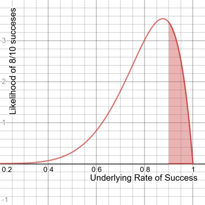
Figure 2-3. The area between 90% and 100%, which is 22.5%
As we did with the binomial distribution, we can use SciPy or build from scratch to implement the beta distribution. Let’s start with SciPy. Every continuous probability distribution has a cumulative density function (CDF) which calculates the area up to a given x value. Let’s say I wanted to calculate the area up to 90% (0.0 to .90) as shaded in Figure 2-4.

Figure 2-4. Calculating the area up to 90% (0.0 to .90)
It is easy enough to use SciPy with its beta.cdf() function, and the only parameters I need to provide are the x value, the number of successes a, and the number of failures b as shown in Example 2-11.
Example 2-11. Beta distribution using SciPy
from scipy.stats import beta

a = 8
b = 2

p = beta.cdf(.90, a, b)

# 0.7748409780000001
print(p)
So according to our calculation above, there is a 77.48% chance the underlying probability of success is 90% or less.
How do we calculate the probability of success being 90% or more as shaded below in Figure 2-5?
Figure 2-5. The probability of success being 90% or more
Our CDF only calculates area to the left of the cutoff, not the right. Think about our rules of probability, and with a probability distribution the total area under the curve is 1.0. If we want to find the opposite probability of an event (greater than .90 as opposed to less than .90), just subtract the probability of being less than .90 from 1.0, and the remaining probability will reflect being greater than .90. Here’s a visual demonstrating how we do this subtraction in Figure 2-6.

Figure 2-6. Finding the probability of success being greater than 90%
Example 2-12 shows how we calculate this subtraction operation in Python.
Example 2-12. Beta distribution using SciPy
from scipy.stats import beta

a = 8
b = 2

p = 1.0 - beta.cdf(.90, a, b)

# 0.22515902199999993
print(p)
So this means out of 8/10 successful engine tests, there is only a 22.5% chance the underlying success rate is 90% or greater. But there is about a 77.5% chance it is less than 90%. The odds are not in our favor here that our tests were successful, but we could gamble on that 22.5% chance with more tests if we are feeling lucky. If our CFO granted funding for 26 more tests resulting in 30 successes and 6 failures, here is what our Beta distribution would look now in Figure 2-7.

Figure 2-7. Beta distribution after 30 successes and 6 failures
Notice our distribution became narrower, thus becoming more confident that the underlying rate of success is in a smaller range. Unfortunately our probability of meeting our 90% success rate minimum has only decreased, going from 22.5% to 13.16% as shown in Example 2-13.
Example 2-13. Beta distribution using SciPy
from scipy.stats import beta

a = 30
b = 6

p = 1.0 - beta.cdf(.90, a, b)

# 0.13163577484183708
print(p)
At this point, it might be a good idea to walk away and stop doing tests, unless you want to keep gambling against that 13.16% chance and hope the peak moves to the right.
Last but not least, how would we calculate an area in the middle? What if I want to find the probability my underlying rate of success is between 80% and 90% as shown in Figure 2-8?
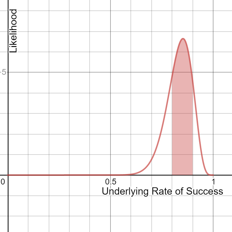
Figure 2-8. Probability the underlying rate of success is between 80% and 90%
Think carefully how you might approach this. What if we were to subtract the area behind .80 from the area behind .90 like in Figure 2-9?
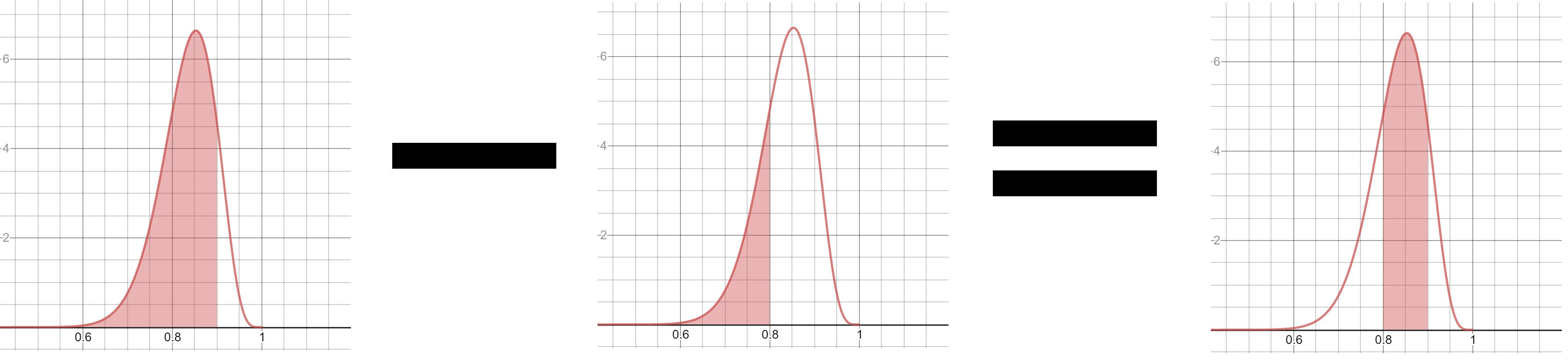
Figure 2-9. Obtaining the area between .80 and .90
Would that not give us the area between .80 and .90? Yes it would, and it would yield an area of .3386 or 33.86% probability. Here is how we would calculate it in Python in Example 2-14.
Example 2-14. Beta distribution using SciPy
from scipy.stats import beta

a = 8
b = 2

p = beta.cdf(.90, a, b) - beta.cdf(.80, a, b)

# 0.33863336200000016
print(p)
The beta distribution is a fascinating tool to measure the probability of an event occuring versus not occurring, based on a limited set of observations or a starting odds ratio quantifying our belief. It allows us to reason about probabilities of probabilities, and we can update it as we get new data. We can also use it for hypothesis testing, but we will put more emphasis on using the normal distribution and t-distribution for that purpose in the next chapter.
Beta Distribution from Scratch
If you are curious how to build a beta distribution from scratch, you will need to re-use the factorial() function we used for the binomial distribution as well as the approximate_integral() function we built in the last chapter.
Just like we did in the previous chapter, we pack rectangles under the curve for the range we are interested in as shown in Figure 2-10?
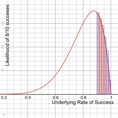
Figure 2-10. Packing rectangles under the curve to find the area/probability
This is just using 6 rectangles and we will get better accuracy if we were to use more rectangles. Let’s implement the beta_distribution() from scratch and integrate 1000 rectangles between .9 and 1.0 as shown in Example 2-15.
Example 2-15. Beta distribution from scratch
# Factorials multiply consecutive descending integers down to 1
# EXAMPLE: 5! = 5 * 4 * 3 * 2 * 1
def factorial(n: int):
    f = 1
    for i in range(n):
        f *= (i + 1)
    return f


def approximate_integral(a, b, n, f):
    delta_x = (b - a) / n
    total_sum = 0

    for i in range(1, n + 1):
        midpoint = 0.5 * (2 * a + delta_x * (2 * i - 1))
        total_sum += f(midpoint)

    return total_sum * delta_x

def beta_distribution(x: float, alpha: float, beta: float) -> float:
    if x < 0.0 or x > 1.0:
        raise ValueError("x must be between 0.0 and 1.0")

    numerator = x ** (alpha - 1.0) * (1.0 - x) ** (beta - 1.0)
    denominator = (1.0 * factorial(alpha - 1) * factorial(beta - 1)) / (1.0 * factorial(alpha + beta - 1))

    return numerator / denominator


greater_than_90 = approximate_integral(a=.90, b=1.0, n=1000, f=lambda x: beta_distribution(x, 8, 2))
less_than_90 = 1.0 - greater_than_90

print("GREATER THAN 90%: {}, LESS THAN 90%: {}".format(greater_than_90, less_than_90))
You will notice with the beta_distribution() function, we provide a given probability x, an alpha value quantifying successes, and a beta value quantifying failures. The function will return how likely we are to observe a given likelihood x. But again, to get a probability of observing probability x we need to find an area within a range of x values. Thankfully, we have our approximate_integral() function defined and ready to go from the last chapter. We can calculate the probability that the success rate is greater than 90%, as well as less than 90% as shown in the last few lines above.
Conclusion
We covered a lot in this section! We not only covered the fundamentals of probability, its logical operators, and Bayes Theorem but we introduced probability distributions including the binomial and beta distributions. In the next chapter we will cover one of the more famous distributions, the normal distribution, and how it relates to hypothesis testing.
If you want to learn more about Bayesian probability and statistics, a great book is Bayesian Statistics the Fun Way by Will Kurt. There are also interactive Katacoda scenarios available on the O’Reilly platform.
Exercises
-
There is a 30% chance of rain today, and a 40% chance your umbrella order will arrive on time. You are eager to walk in the rain today and cannot do so without either!
What is the probability it will rain AND your umbrella will arrive?
-
There is a 30% chance of rain today, and a 40% chance your umbrella order will arrive on time.
You will only be able to run errands if it does not rain or your umbrella arrives.
What is the probability it will not rain OR your umbrella arrives?
-
There is a 30% chance of rain today, and a 40% chance your umbrella order will arrive on time.
However, you found out if it rains there is only 20% chance your umbrella will arrive on time.
What is the probability it will rain and your umbrella will arrive on time?
-
You have 137 passengers booked on a flight from Las Vegas to Dallas. However it is Las Vegas on a Sunday morning and you estimate each passenger is 40% likely to not show up.
You are trying to figure out how many seats to overbook so the plane does not fly empty.
How likely is it at least 50 passengers will not show up?
-
You flipped a coin 19 times and got heads 15 times and tails 4 times.
Do you think this coin has any good probability of being fair? Why or why not?