4.1.1 Vector Spaces

The term vector has more than one meaning, depending on the context in which it is used. We saw in “2.1 Coordinates And Vectors” that vectors can describe how to go from a point $A$ to another point $B$. To characterize this displacement, we need a magnitude and a direction. In computer science, a vector is an ordered list of numbers.

In this book, when I talk about vectors, I mean free vectors represented in a Cartesian coordinate system, with the origin as the initial point. These vectors can be represented by ordered lists of numbers corresponding to the terminal point coordinates.

Axioms

The mathematical definition is a bit broader however. In pure mathematics, vector refers to objects that can be added and multiplied by a scalar. These two operations must satisfy some rules called axioms. Here are these axioms:

• $?+?=?+?$

• $(?+?)+?=?+(?+?)$

• $?+0=?$

• For all $?$, there is an element $-?$ so that: $?+(-?)=0$

• $(c+d)?=c?+d?$

• $c(?+?)=c?+c?$

• $c\left(d?\right)=\left(cd\right)?$

• $1?=?$

A set of vectors that satisfies these axioms is called a vector space.

Let’s see some vector types that we already know from the first part of the book, and look at how the two operations addition and scalar multiplication are executed.

4.1.2 Coordinate Vectors

As you have seen, what we call coordinate vectors are ordered lists of numbers corresponding to coordinates.

Indexing

Since we’ll use Numpy to get more insight about vectors, let’s recap few basic things that you can do to interact with vectors.

Indexing refers to the process of getting a vector element (one of the values from the vector) using its position in the vector (its index). In other words, the index of an element in a vector is its position in the vector.

For instance, let’s consider the following vector:

The index of the element 0.3 is 0, the index of 0.8 is 1 and so on. Let’s create this vector with Numpy and try some indexing.

v = np.array([0.3, 0.8, 0.2, 0.9])
v

array([0.3, 0.8, 0.2, 0.9])

Indexing is done using square brackets ([]). For instance, you can get the first element of v with:

v[0]

0.3

Or the element 1 with:

v[1]

0.8

It is also possible to get multiple elements. For instance, to get the elements from 1 (included) to 3 (excluded):

v[1:3]

array([0.8, 0.2])

4.2.1 Unit Vectors

We call unit vector vectors that have a length of 1 (more details on vector length were given in “2.1 Coordinates And Vectors”).

4.2.2 Basis Vectors

We have seen that vectors can be represented as arrows going from the origin to a point that has coordinates corresponding to the numbers stored in an ordered list of coordinates, as shown in Figure 4-1.

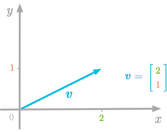
Figure 4-1. Relation between geometric representation of vectors and list of numbers.

The geometric representation shown in Figure 4-1 imply that we take a reference: the directions given by the two axes $x$ and $y$. We call basis vectors the special vectors that have a length of 1 (unit vectors) and the directions used as reference. These vectors point in the direction of the axes and are unit vectors (they have a length of 1). For instance, in Figure 4-2, the basis vectors $i$ and $j$ point in the direction of the axis $x$ and $y$ respectively.

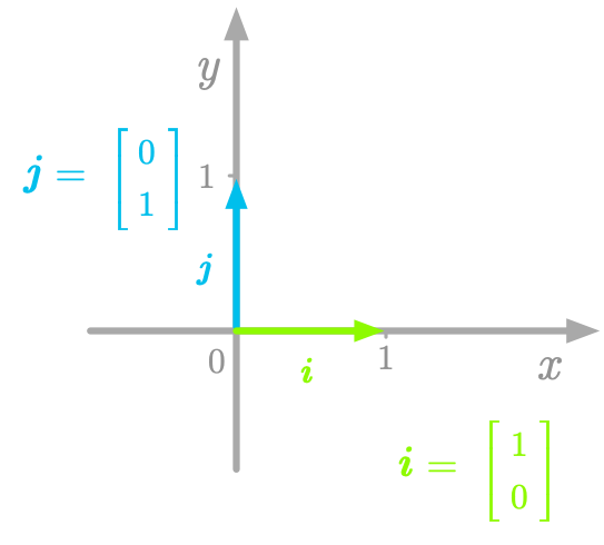
Figure 4-2. The basis vectors in the Cartesian plane.

?? Wait linear combination for this ??

Any vector can be thought of as a scaled version of basis vectors. For instance, in Figure 4-3, we can consider the vector $v$ a stretched version of the basis vector $i$: it is scaled by a factor of 2.

Figure 4-3. The vector $v$ can be considered a scaled version of the basis vector $i$.

The basis of our vector space is very important because the values used to characterize the vectors are relative to this basis. By the way, you can choose different basis vectors (you can see an example in Figure 4-4). Keep in mind that vector coordinates depend on an implicit choice of basis vectors.

Figure 4-4. New basis vectors.

This shows that a space exists independently of the coordinate system we are using. The coordinate values corresponding to a vector in this space depends on the basis we choose.

4.2.3 Zero Vectors

A zero vector or null-vector is a vector of length 0. Adding the zero vector doesn’t change a vector.

4.2.4 Row and Columns Vectors

We can distinguish vectors according to their shape. In column vectors, the numbers are organized as a column:

In row vectors, they are organized as a row:

The convention is to use column vectors to list point coordinates.

Numpy is great to work with vectors. We’ll use this library to get practical insights about linear algebra. In Numpy, the function array() can be used to create vectors. Let’s try it:

v_row = np.array([1, 2, 3])
v_row

array([1, 2, 3])

We have created the Numpy equivalent of a vector: an array. You can use the property shape to check the shape of the array:

v_row.shape

(3,)

We can see that there is only one dimension (one number). This is because this is a vector. Numpy doesn’t distinguish between row and column vectors. To make this distinction, you would need to create a matrix with one column or one row (see in [Link to Come]).

4.2.5 Orthogonal Vectors

Two vectors are called orthogonal when they run in perpendicular directions. You can see a geometric example of two orthogonal vectors in Figure 4-5.

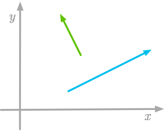
Figure 4-5. Two orthogonal vectors.

If the length of both orthogonal vectors is 1 (that is, if they are unit vectors), then they are called orthonormal.

4.3.1 Scalar Multiplication

Scalar multiplication is the operation of multiplying a scalar with a vector. When multiplied by a scalar, a vector gives another vector (a scaled version of the initial vector). So, multiplying a vector by a scalar is like rescaling this vector. For instance, in Figure 4-6, the vector $?$ is rescaled when multiplied by 1.3:

Figure 4-6. Multiplication of the vector $?$ by a number (1.3).

Let’s represent $v$ as a coordinate vector:

The scalar multiplication of $v$ will give us the following result:

Multiplying the vector $?$ by a scalar corresponds to multiply each element of this vector by the scalar. With our example, both dimensions, x and y, are scaled by the scalar.

We can use Numpy to do scalar multiplication:

v = np.array([2, 1])
v

array([2, 1])

1.3 * v

array([2.6, 1.3])

4.3.2 Vector Addition

Adding two vectors gives another vectors.

Let’s take two vectors ${?}_1$ and ${?}_2$.

Figure 4-7. Geometrical representation of the two vectors ${?}_1$ and ${?}_2$.

Figure 4-7 shows their geometric representation.

Here is how these two vectors can be added together. As shown in Figure 4-8, adding them can be understood as changing the position from the origin to the terminal point of the first vector; from this terminal point, the change in position of the second vector is applied.

Figure 4-8. Adding the vectors ${?}_1$ and ${?}_2$ gives another vector.

For each dimension, the coordinate of the new vector is the sum of the coordinates of the two vectors we added together. If we consider the coordinates of these geometric vectors, we can see how these operations can be done. In Figure 4-8, we had the vectors $v_1$ and $v_2$ that are defined by the following coordinates:

and

The first value corresponds to the x-coordinate and the second value to the y-coordinate. The vector resulting of the addition of $v_1$ and $v_2$ has an x-coordinate that corresponds to the sum of the x-coordinates of both vectors and the same for its y-coordinate:

Let’s do this vector addition with Numpy:

v1 = np.array([2, 1])
v1

array([2, 1])

v2 = np.array([2, 0])
v2

array([2, 0])

v1 + v2

array([4, 1])

Example

If your data is stored in vector form, you can efficiently create a new vector that corresponds to the sum of two other vectors. For instance, let’s say that you are working on a demographic dataset where one vector corresponds to the number of male children and another vector to the number of female children. You can calculate the total number of children for each data sample by adding the two vectors together.

4.3.3 Using Addition and Scalar Multiplication

You can think of each number of a coordinate vector as a scalar that scales the basis vectors (for instance, $i$ and $j$ in the two-dimensional Cartesian plane). For example, coordinates of the vector $v$ shown in Figure 4-1 correspond to the sum of the vector $i$, scaled by the $x$ coordinate of $v$, and the vector $j$, scaled by the $y$ coordinate of $v$. So we have:

4.3.4 Transposition

We have seen that vector values can be organized as rows or as columns. The transpose of a vector is an operator that transforms a row vector into a column vector or the opposite. It is denoted as the superscript letter $\text{T}$ (for instance, ${?}^{\text{T}}$).

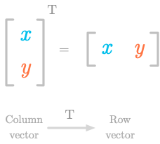
Figure 4-9. The transpose of a column vector is a row vector.

For instance, Figure 4-9 shows the transposition of a two-dimensional vector from column to row. So you can have:

and

With Numpy, the transpose of a vector is given by the simple letter T. However, since the distinction between row and column vector is not made, this will have no effect on one-dimensional arrays:

v = np.array([1, 2])
v

array([1, 2])

v.T

array([1, 2])

4.3.5 Operations on Other Vector Types - Functions

Other mathematical entities can be considered vectors if they satisfy the axioms listed in “4.1.1 Vector Spaces”.

Using this definition, functions can be considered vectors. Let’s try adding and multiplying functions.

Let’s take the following functions:

and

Now, plot these two functions:

# create x and y vectors
x = np.linspace(-2, 2, 100)
y = x ** 2

y1 = 3 * np.sin(x)

# choose figure size
plt.figure(figsize=(6, 6))

# Assure that ticks are displayed with a step equal to 1
ax = plt.gca()
ax.xaxis.set_major_locator(ticker.MultipleLocator(1))
ax.yaxis.set_major_locator(ticker.MultipleLocator(1))

# draw axes
plt.axhline(0, c='#A9A9A9')
plt.axvline(0, c='#A9A9A9')

# assure x and y axis have the same scale
# plt.axis('equal')

plt.plot(x, y, label="$x^2$")
plt.plot(x, y1, label="$3 sin(x)$")
plt.legend()

Figure 4-10. Plot of the functions $f\left(x\right)$ and $g\left(x\right)$.

Now, let’s plot the addition of these two functions:

# choose figure size
plt.figure(figsize=(6, 6))

# Assure that ticks are displayed with a step equal to 1
ax = plt.gca()
ax.xaxis.set_major_locator(ticker.MultipleLocator(1))
ax.yaxis.set_major_locator(ticker.MultipleLocator(1))

# draw axes
plt.axhline(0, c='#A9A9A9')
plt.axvline(0, c='#A9A9A9')

plt.plot(x, y, label="$x^2$")
plt.plot(x, y1, label="$3 sin(x)$")
plt.plot(x, y + y1, label="$x^2 + 3sin(x)$")
plt.legend()

Figure 4-11. Adding the functions $f\left(x\right)$ and $g\left(x\right)$.

We can see in Figure 4-11 that adding $f\left(x\right)$ and $g\left(x\right)$ gives another function ($x^2+3sin\left(x\right)$).

We can do the same for scalar multiplication. For instance, let’s take $f\left(x\right)$ and multiply it by -3:

# choose figure size
plt.figure(figsize=(6, 6))

# Assure that ticks are displayed with a step equal to 1
ax = plt.gca()
ax.xaxis.set_major_locator(ticker.MultipleLocator(1))
ax.yaxis.set_major_locator(ticker.MultipleLocator(1))

# draw axes
plt.axhline(0, c='#A9A9A9')
plt.axvline(0, c='#A9A9A9')

plt.plot(x, y, label="$x^2$")
plt.plot(x, y * -3, label="$-3x^2$")
plt.legend()

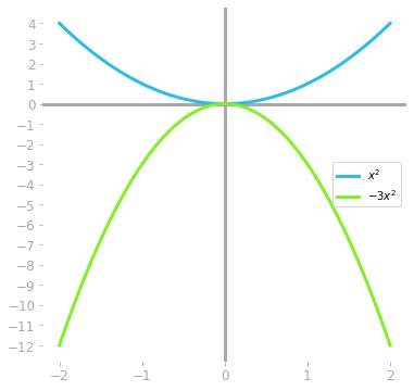
Figure 4-12. Multiplying the functions $x^2$ by $-3$.

It shows the plurality of what vectors can be. You can imagine various vector spaces: the vectors only have to satisfy the axioms. This is really just a mathematical convention.

Vectors are central to linear algebra. In this section of the book, I will represent vectors as coordinate vectors, that is, ordered lists of values. You can think of these as referring to arrow coordinates in a Cartesian plane.

What you will learn in this book about linear algebra can be applied to any vectors from this general definition. However, these concepts are usually explained through applying them to a single kind of vector. The definitions and proofs in math textbooks are more abstract because they have to encompass any type of vectors (thus, any type of objects that satisfy the axioms).

4.4.1 Definitions

Interpreting the norm as the vector length is not necessarily straightforward. This depends on how you define a distance. There are multiple norms that are calculated differently. A mathematical entity can be called norm only if it respects the following rules:

Triangle Inequality

Norms respect the rule of triangle inequality, according to which the norm of the sum of two vectors is less than or equal to the norm of the first vector summed with the norm of the second vector.

We can write this mathematically as following:

$$∥?+?∥\le ∥?∥+∥?∥$$

As shown graphically in Figure 4-13, triangle inequality means simply that the shortest path between two points is a line.

Figure 4-13. Illustration of triangle inequality.

With Numpy, the norm of a vector can be calculated with the function np.linalg.norm(). Let’s take the example corresponding to Figure 4-13:

v1 = np.array([2, 1])
v2 = np.array([1, 1])

np.linalg.norm(v1 + v2)

3.605551275463989

np.linalg.norm(v1) + np.linalg.norm(v2)

3.6502815398728847

The results show that the norm of $v1$ summed with the norm of $v2$ is larger than the norm of $v1+v2$.

4.4.2 Examples of Norms

Every function that satisfies the rules from the last section can be called a norm. This implies that there is more than one kind of norm.

In machine learning and deep learning, it is important to be able to compare vectors. Norms provide a way to do that; different kind of norms can be used, and each has pros and cons.

Many norms fall into the category of the p-norm, which means the sum of the absolute value of each dimension raised to the power of a value $p$. The result of this sum is raised to the power of $\frac{1}{p}$. It may be easier to read the mathematical formula:

with $m$ the number of elements in the vector, $x$ our vector, $i$ the current vector element.

Let’s split this equation to be sure that everything is clear:

• $|x_i|$ corresponds to the absolute value of the $i$th element of the vector.

• $|x_i{|}^p$: the absolute value is raised to the power of $p$.

• ${\sum }_i^m{\left|x_i\right|}^p$ we calculate the sum of all powered absolute values from the vector $x$ from the first to the $m$ element (you can see more details on the sum notation in Sigma notation).

• $({\sum }_i^m|x_i{{|}^p)}^{\frac{1}{p}}$: we take the power $\frac{1}{p}$ of this result.

Different values of $p$ give different norms: $p=0$ is called the $L^0$ norm, $p=1$ is called the $L^1$ norm, $p=2$ is called the $L^2$ norm. These three norms are the more common ones.

v = np.array([1, 0, 0, -1.532, 230, 0.23, 1.7])
v

array([  1.   ,   0.   ,   0.   ,  -1.532, 230.   ,   0.23 ,   1.7  ])

np.sum(v != 0)

5

np.linalg.norm(v, 0)

5.0

$L^1$ Norm

The $L^1$ norm is a function returning the sum of the absolute value of the coordinates:

$$\begin{array}{cc}\hfill {∥?∥}_1& =(\sum _i^m|{?}_i{{|}^1)}^{\frac{1}{1}}\hfill \\ \\ & =\sum _i^m\left|{?}_i\right|\hfill \end{array}$$

with $m$ the number of elements in the vector, $i$ the current element, and $x$ the vector.

Taxicab distance

The $L^1$ norm is also called the Manhattan distance or the taxicab distance because of the displacement of a taxi in a street grid, like in Manhattan.

Figure 4-14. With the Manhattan distance, each path has the same length.

As illustrated in Figure 4-14, a taxi driver would prefer to take the yellow diagonal path if it would be possible. It is because the $L^2$ norm represents the physical world: this is different when we use the the $L^2$ norm.

REF: https://en.wikipedia.org/wiki/Taxicab_geometry

For instance, we can see in Figure 4-15 the $L^1$ norm of the vector $v$.

Figure 4-15. L1 norm of the vector $v$.

The $L^1$ norm can be calculated with Numpy as follows:

v1 = np.array([2, 1])
v1

array([2, 1])

np.linalg.norm(v1, 1)

3.0

$L^2$ Norm

The $L^2$ norm is even more used in machine learning and deep learning than the $L^1$ norm. It is also called the Euclidean distance. The vector length measured with the $L^2$ norm corresponds to the physical distance in the real world, which is a consequence of the Pythagorean theorem (as we have seen in “2.2 Distance formula”). The formula is as follows:

$$\begin{array}{cc}\hfill {∥?∥}_2& =(\sum _i^m|{?}_i{{|}^2)}^{\frac{1}{2}}\hfill \\ \\ & =\sqrt{{\sum }_i^m{\left|{?}_i\right|}^2}\hfill \\ \hfill & =\sqrt{{\sum }_i^m{?}_i^2}\hfill \end{array}$$

with $m$ the number of elements in the vector, $i$ the current element, and $x$ the vector.

We don’t need to take the absolute value of coordinates since they are raised to the power of two.

For instance, we can see in Figure 4-16 the $L^2$ norm of the vector $v$.

Figure 4-16. L2 norm of the vector $v$.

It is possible to use Numpy to calculate the $L^2$ norm:

np.linalg.norm(v1, 2)

2.23606797749979

v = np.array([1, 0, 0, -1.532, 230, 0.23, 1.7])
v

array([  1.   ,   0.   ,   0.   ,  -1.532, 230.   ,   0.23 ,   1.7  ])

np.linalg.norm(v, np.inf)

230.0

4.4.3 Norm Representations

We have seen that multiple types of norms can be used to measure the length of a vector. Norms have different characteristics that are visible when we plot them.

The Unit Circle

The unit circle is a shape where every point has a distance of 1 from the center. According to the kind of distance we use ($L^1$, $L^2$, max…), this shape is different.

In Figure 4-17, some points with a distance of 1 from the origin have been represented according to the norm.

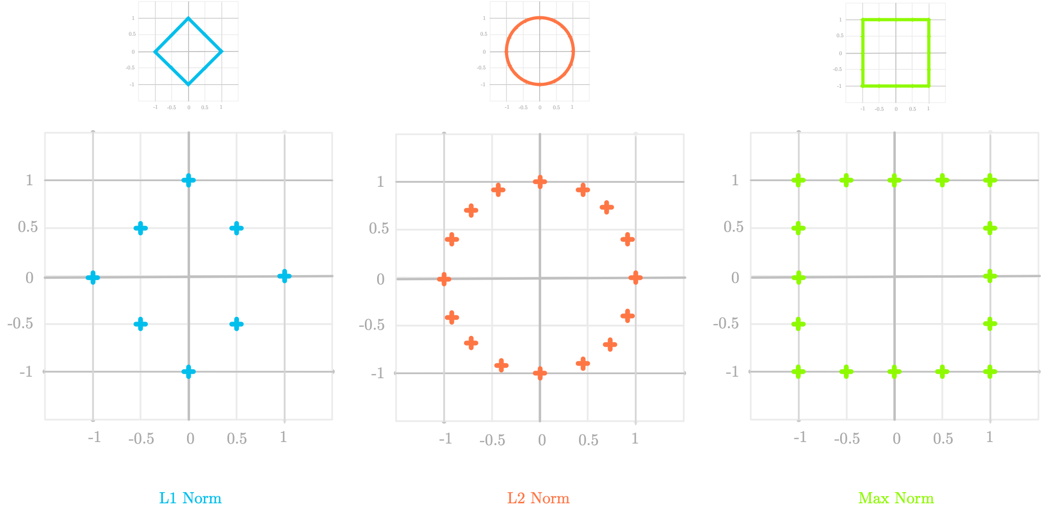
Figure 4-17. Comparison of unit shapes for the $L^1$, $L^2$ and max norm.

$L^1$ Norm

For instance, let’s calculate the $L^1$ norm of the point with coordinates (0.5, 0.5) from the left panel. We have:

$$\sum _i^m|{?}_i|=|0.5|+|0.5|=1$$

If we take another point, for instance the point with coordinates (0, 1) we have also:

$$\sum _i^m|{?}_i|=|1|+|0|=1$$

The small panel shows that if we take a lot of points with a distance of 1 from the origin, we have not a circle but a diamond shape.

$L^2$ Norm

The middle panel in Figure 4-17 shows the unit shape for the $L^2$ norm, which is a circle. This corresponds to what we expect in the physical world (where the word “distance” refers to the $L^2$ distance), where every point on a circle has the same distance from the center.

Max Norm

Finally, in the right panel, every point where the maximum of the two coordinate is 1 is on the unit shape. For example, the point of coordinate (0.5, 1) has a max norm of 1 and is thus on the unit shape.

Contour Plot

Another way to visualize these norm is to use a contour plot. The following code shows in Figure 4-18 the contour plot of both the $L^1$ and $L^2$ norms.

import seaborn as sns

x = np.linspace(-10, 10, 50)
y = np.linspace(-10, 10, 50)

X, Y = np.meshgrid(x, y)

def cost_function_l1(X, Y):
    Z = np.abs(X) + np.abs(Y)
    return Z

def cost_function_l2(X, Y):
    Z = np.sqrt(np.square(X) + np.square(Y))
    return Z


Z_1 = cost_function_l1(X, Y)
Z_2 = cost_function_l2(X, Y)

plt.figure(figsize=(8, 8))

# Assure that ticks are displayed with a step equal to 1
ax = plt.gca()
ax.xaxis.set_major_locator(ticker.MultipleLocator(1))
ax.yaxis.set_major_locator(ticker.MultipleLocator(1))

# draw axes
plt.axhline(0, c='#A9A9A9')
plt.axvline(0, c='#A9A9A9')

# assure x and y axis have the same scale
plt.axis('equal')

plt.subplot(221)
plt.title("L1 Norm")
plt.contour(X, Y, Z_1)

plt.subplot(222)
plt.title("L2 Norm")
plt.contour(X, Y, Z_2)

Figure 4-18. Contour plot of the $L^1$ and $L^2$ norms.

4.5.1 Definition

The dot product between two vectors $v_1$ and $v_2$, denoted by the symbol $·$, is defined as the sum of the product of each pair of elements. More formally, it is expressed as:

with $m$ the number of elements in the vectors $v_1$ and $v_2$ (they have to contain the same number of elements) and $i$ the index of the current vector element.

Let’s take an example. We have the following vectors:

and

The dot product of these two vectors is defined as:

Note that we take the transpose of the first vector to ensure that the shapes match (however, using vectors and not matrices in Numpy, you won’t need to do that). The dot product between $v_1$ and $v_2$ is 35.

Let’s see how we do this Numpy:

v1 = np.array([2, 4, 7])
v1

array([2, 4, 7])

v2 = np.array([5, 1, 3])
v2

array([5, 1, 3])

Numpy arrays have a method dot() that do exactly what we want.

v1.dot(v2)

35

It is also possible to use the following equivalent syntax:

np.dot(v1, v2)

35

Or, with Python 3.5+, it is also possible to use the @ operator:

v1 @ v2

35

i = np.array([0, 1])
j = np.array([1, 0])
i @ j

0

4.5.2 Geometric interpretation

We could wonder how the dot product between two vectors is interpreted when apply to geometric vectors. We have seen the geometric interpretation of addition of vectors or multiplication by scalars, but what about the dot product?

Let’s take the two following vectors:

and

The dot product of these two vectors ($v_1·v_2$) gives a scalar. Let’s start by calculating it:

What is the meaning of this value? Well, it is related to the idea of projecting $v_1$ onto $v_2$. As shown in Figure 4-19, the projection of $v_1$ on the line with the direction of $v_2$ is like the shadow of the vector $v_1$ on this line.

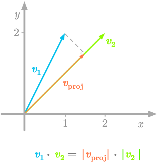
Figure 4-19. The dot product can be seen as the length of $v_2$ multiplied by the length of the projection.

The value of the dot product (6 in our example) corresponds to the multiplication of the length of $v_2$ (its norm: $|v_2|$) and the length of the projection of $v_1$ on $v_2$ ($\left|\right|v_{\text{proj}}\left|\right|$).

Let’s do the math. We have:

As we will see in [Link to Come], the projection of $v_1$ onto $v_2$ is:

So the length of $v_{\text{proj}}$ is:

Finally, the multiplication of the length of $v_2$ and the length of the projection is:

This is the value we found with the dot product.

Special cases

The value that you obtain with the dot product tells you the relation between the two vectors. As shown in Figure 4-20, if this value is positive, the vectors are a going in the same way. If it is negative, the vectors are going in opposite ways. If it is zero, the vectors are orthogonal.

Figure 4-20. Link between the value of the dot product and the vector directions. This value is positive if the two vectors have the same direction, negative if they have an opposite direction, and zero if they are orthogonal.

4.5.3 Properties

The dot product has the following properties. Let’s take the following example vectors to illustrate them:

v1 = np.array([2, 4, 7])
v2 = np.array([1, 3, 2])
v3 = np.array([3, 5, 5])

v1 @ (v2 + v3)

89

(v1 @ v2) + (v1 @ v3)

89

v1 @ v2

28

v2 @ v1

28

4.5.4 Hands-on Project: Vectorizing the Squared $L^2$ Norm with the Dot Product

In this Hands-on Project, we will see why the squared $L^2$ norm can be easily vectorized, improving computational efficiency.

Let’s take the vector $v$:

Remember from the formula of the squared $L^2$ norm (“Squared L2 Norm”) that we have to calculate the sum of the squared vector elements:

with $m$ the number of elements in the vector, $i$ the current element, and $x$ the vector.

Let’s calculate the squared $L^2$ norm of our vector $v$. We have:

Now, let’s use the dot product to calculate the squared $L^2$ norm. We have seen that:

If we apply this to our vector $v$ we have:

We end up with the same result.

Let’s use the dot product from Numpy to calculate the squared $L^2$ norm of our vector $v$:

v = np.array([2, 1.3, 4, 7.2])
v

array([2. , 1.3, 4. , 7.2])

np.linalg.norm(v, 2) ** 2

73.53000000000002

v @ v.T

73.53

The difference between the two approaches is that vectorization doesn’t use for loops. At the hardware level, vectorized code can be optimized and computations can be ran in parallel¹.