
CHAPTER 7
Updating a Pivot Table
Most pivot tables are based on source data that continues to change; new records or fields may be added to the source data, existing records are modified, or the source data file is moved to a new location. You want to ensure that your pivot table contains the latest available data and is correctly connected to the source data.
To reproduce the environment in which they were created, sample files must be stored in a C:\_Work folder, for testing. If a different folder is used, the connections will be broken. Create this folder on your computer's C: drive, and then copy all the sample files to it. Depending on your security settings, you may see a security warning when opening some sample files. To work with the file, you can enable the data connections.
Except where noted, the problems in this chapter are based on the Sales_07.xlsx sample workbook.
7.1. Using Source Data: Locating the Source Excel Table
Problem
You've been asked to make changes to the pivot table on the ProductSales worksheet, and you'd like to find the Excel Table used as its source data. Several Excel Tables are in the workbook, and you aren't sure which one was used. This problem is based on the Sales07.xlsx sample workbook.
Solution
You can locate the Excel Table that contains the source data by following these steps:
- Select a cell in the pivot table, and on the Ribbon, click the Options tab.
- In the Data group, click the upper section of the Change Data Source command.
- In the Change PivotTable Data Source dialog box, you can see the source table or range in the Table/Range box. This may be a table name, such as
Sales_Eastor a worksheet reference, such as
Sales_East!$A$1:$O$500
- On the worksheet, you can see the source range, surrounded by a moving border.
- Click OK, or Cancel, to close the dialog box.
How It Works
In most cases, the source range is visible, and surrounded by a moving border. If the source range is not activated, it may be on a hidden worksheet. Follow these steps to unhide the sheet:
- Right-click any worksheet tab, and then click Unhide.
- In the Unhide Sheet list, select the sheet you want to make visible, and then click OK.
Tip If the sheet name is not on the list of hidden sheets, it may have been hidden programmatically or removed from the workbook.
If a range name appears in the Table/Range box and the range is not selected, you can check the name definition, to find its location, and to see if there are any problems with the name definition:
- On the Ribbon, click the Formulas tab, and in the Defined Names group, click Name Manager.
- In the Name Manager, the Excel Tables and defined names are listed (see Figure 7-1). Select a name in the list, and in the Refers To box, you'll see the worksheet name on which the range is located.
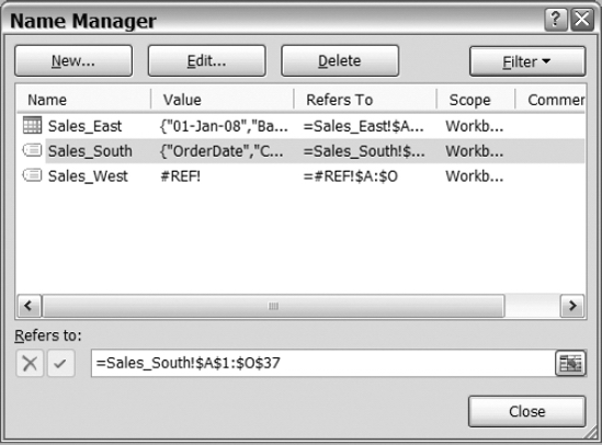
Figure 7-1. Name Manager dialog box
Tip If the Refers To formula for a defined name contains #REF! errors, the worksheet, or some of its cells, may have been deleted.
- If errors are in the formula for a defined name, correct them if possible, or delete the problem name, and then select a new source for the pivot table.
Note The formulas for Excel Tables cannot be changed in the Name Manager. Close the Name Manager, and then make the changes on the worksheet where the Excel Table is located. To add rows or columns, drag the resize handle at the bottom right of the last cell in the Excel Table.
7.2. Using Source Data: Automatically Including New Data
Problem
Your pivot table is based on data in the same Excel file, and you frequently add new records to the source data. Each time you add records, you have to change the source range for the pivot table, to include the new rows.
You would like the source data range to automatically expand to include any new rows and columns. This problem is based on the NewData.xlsx sample workbook.
Solution
When creating a pivot table from Excel data, the best solution is to create a formatted Excel Table from the data, as described in Section 1.4. Then, use the name of the Excel Table as the source for the pivot table. The Excel Table automatically adjusts if records are added or deleted, and the pivot table includes the latest data when it's refreshed.
If you don't want to use a formatted Excel Table, you can use a dynamic range as the pivot table's source. The dynamic range automatically expands to include the new rows and columns. Follow these steps to create a dynamic range, in the sample file:
- On the Orders sheet, select cell A1, which is the top-left cell in the source range. This step isn't necessary, but it helps you by inserting the cell reference in the name definition.
- On the Ribbon, click the Formulas tab, and then in the Defined Names group, click Define Name, to open the New Name dialog box.
- In the Name box, type a name for the dynamic range, for example, PivotSource.
- Leave the Scope setting as Workbook, and add a comment (optional), to describe the name or its purpose.
In the Refers To box, type an OFFSET formula that references the selected cell
=OFFSET(Orders!$A$1,0,0,COUNTA(Orders!$A:$A),COUNTA(Orders!$1:$1))or you can use a nonvolatile formula, which may be more efficient in larger workbooks, where calculation speed is an issue:
= Orders!$A$1:INDEX(Orders!$1:$10000,

     COUNTA(Orders!$A:$A),COUNTA(Orders!$1:$1))
The formula is set to a limit of 10,000 rows, which can be increased if required.
- Click the OK button.
Caution These formulas do not work correctly if other items are in Row 1 or Column A of the Orders worksheet. Those items would be included in the count, and would falsely increase the size of the source range, or they could cause an error when the pivot table is refreshed. Blank cells within the data in the row or column being counted would also cause a problem, reducing the size of the source range. Count a column and row where there is always a value.
After you create the named range, change the pivot table's source to the dynamic range:
- Select a cell in the pivot table, and on the Ribbon, click the Options tab.
- In the Data group, click Change Data Source.
- In the Table/Range box, type the name of the dynamic range, PivotSource in this example, and then click OK.
Tip While in the Table/Range box, delete the existing table or range. Then, to see a list of defined names, press the F3 key. Click a name in the Paste Name dialog box, to select it, and then click OK.
How It Works
The OFFSET function returns a range reference of a specific size, offset from the starting range by a specified number of rows and columns. The function has three required arguments (shown in bold font), and two optional arguments:
=OFFSET(reference,rows,columns,height,width)
In our example
=OFFSET(Orders!$A$1,0,0,COUNTA(Orders!$A:$A),COUNTA(Orders!$1:$1))
the returned range starts in cell A1 on the worksheet named Orders. It is offset zero rows and zero columns. The height of the range is determined by counting the cells that contain data in Column A of the Orders worksheet:
COUNTA(Orders!$A:$A)Note If Column A contains any blank cells within the data range, use a column that does not contain blank cells. Blank cells reduce the count and result in a range that is too small.
The width of the range is determined by counting the cells that contain data in Row 1 of the Orders worksheet:
COUNTA(Orders!$1:$1)
This creates a dynamic range, because if rows or columns are added, the size of the range in the defined name increases.
The INDEX formula is similar, but it creates a range that starts in Cell A1 on the Orders sheet, and ends at the cell referenced by the INDEX function.
= Orders!$A$1:INDEX(Orders!$1:$10000,

     COUNTA(Orders!$A:$A),COUNTA(Orders!$1:$1))
7.3. Using Source Data: Automatically Including New Data in an External Data Range
Problem
In your workbook, you imported a text file that contains billing data, on to the BillingData worksheet. This created an external data range that has a connection to the text file. If new billing records are added to the external file, they appear in the external data range when it's refreshed. However, the pivot table is based on the imported data, but when you refresh the pivot table, the new records don't appear.
You can't create a formatted Excel Table from the external data range, or the connection to the external data will be lost.
This problem is based on the Billing.xlsx sample workbook. Depending on your security settings, you may see a security warning when opening the sample file. To work with the file, you can enable the data connections.
Solution
When you import external data to an Excel worksheet, using the commands in the Get External Data group on the Data tab of the Ribbon, a named External Data Range is created for the imported data. If you base the pivot table on this named range, it expands automatically as new records are added, and the pivot table contains all the data.
When you created a pivot table from the external data, you may have used a reference to range of cells, such as BillingData!$A$1:$J$19, instead of using the external data range's name. If data is added to the external data file, the new data appears in the Excel workbook, when the external data range is refreshed. However, the pivot table continues to use the original range, and the new data is not included in the pivot table when it's refreshed.
Follow these steps to change the pivot table's data source, so it uses the external data range name:
- To see the name of the external data range, right-click a cell in the external data range, and then click Data Range Properties. The range name is shown at the top of the External Data Range Properties dialog box. Click OK to close the dialog box.
- To base the pivot table on this range, select a cell in the pivot table, and then click the Options tab on the Ribbon.
- In the Data group, click Change Data Source.
- Type the external data range's sheet name and table name in the Table/Range box. For example, if the sheet name is BillingData and the external data range name is Billing_1:
BillingData!Billing_1
- Click OK.
7.4. Using Source Data: Moving the Source Excel Table
Problem
Your pivot table is based on a named range in another workbook. Using Windows Explorer, you copied the two workbooks to your laptop, so you could work at home, but when you tried to refresh the pivot table, you got an error message: "Cannot open PivotTable source file...." This problem is based on the SalesData.xlsx and SalesPivot.xlsx sample workbooks.
Solution
You can reconnect the pivot table to the named range, in its new location:
- Open both files—the file with the pivot table, and the file that contains the source data.
- Activate the file that contains the pivot table, and then select a cell in the pivot table.
- On the Ribbon, click the Options tab, and in the Data group, click Change Data Source.
- While the Change PivotTable Data Source dialog box is open, on the Ribbon, click the View tab. Click Switch Windows, and select the workbook that contains the source data.
- Select the table that contains the source data, and then click OK.
Note When you copy the files back to your desktop computer, you'll have to follow the same steps to reconnect them.
When you create a pivot table that's based on data in another workbook, and that workbook is in a different folder, the folder path is stored as part of the source range. When you copy the files to a different computer, or move the data source file to a different folder, the pivot table can't connect to it.
To prevent this problem, create and save the pivot table file in the same folder as the data source file. Then, you can move the two files to any other location, keeping the two files together, and when refreshing, the pivot table looks for the data source file in its current folder.
7.5. Using Source Data: Changing the Source Excel Table
Problem
Your pivot table is based on an Excel Table in the same workbook as the pivot table. You want to change the source to a table in another workbook. This problem is based on the Central.xlsx and East.xlsx sample workbooks.
Solution
Follow these steps to change the source for the pivot table in the Central.xlsx workbook to the Excel Table in the East.xlsx workbook:
- Open both workbooks—the file with the pivot table (
Central.xlsx), and the file that contains the new source data (East.xlsx). - Select a cell in the pivot table, and then on the Ribbon, click the Options tab.
- In the Data group, click Change Data Source.
- While the Change PivotTable Data Source is open, on the Ribbon, click the View tab. Click Switch Windows, and then select the workbook that contains the new source data.
Select the range for the source data, and the Range reference is created, including the workbook name, for example:
[East.xlsx]Sales_East!$A$1:$G$21If you select an Excel Table or named range in the other workbook, the name won't be shown in the Range reference, so you can modify the reference to include it. For example, if the workbook contains an Excel Table named EastData, you'd type
[East.xlsx]Sales_East!EastData
For a workbook-level range named PivotRange, you'd remove the square brackets and the sheet reference, and then type
East.xlsx!EastData
- Click OK.
Note The workbook that contains the source data can be open or closed when you're using or refreshing the pivot table. However, if the reference is to an Excel Table, or to a dynamic range in the other workbook, that workbook must be open to refresh the pivot table.
7.6. Using Source Data: Locating the Source Access File
Problem
You inherited a pivot table that's based on a Microsoft Access query. When you click the Change Data Source command, you can see the connection name in the Change PivotTable Data Source dialog box. However, you can't see the name of the Access file, or tell which query was used to create the pivot table. You'd like to find out which database and query were used, so you can make a change to the query. This problem is based on the Shipments.xlsx and Shipments.accdb sample files.
Solution
You can view the connection properties to find the Access file name and path:
- In the
Shipments.xlsxfile, select a cell in the pivot table, and then on the Ribbon, click the Data tab. - In the Connections group, click Properties.
- In the Connection Properties dialog box, you can see the Connection name at the top. Click the Definition tab.
- In the Connection File box, you can see the name and path of the database. In the Command Text box is the name of the Access query.
- Click Cancel to close the Connection Properties dialog box.
7.7. Using Source Data: Changing the Source Access File
Problem
You created a pivot table from an Access query, and the Access file was moved to a different directory. When you tried to refresh the pivot table, you got the error message "Could not find file 'C:\_WorkShipments.accdb'." When you clicked OK, a dialog box appeared with the heading, "Please Enter Microsoft Office Access Database Engine OLE DB Initialization Information." Just reading that heading makes you tired, and you'd like to find a simple way to reconnect the pivot table to the database. This problem is based on the Shipments.xlsx and Shipments.accdb sample files.
If the source database has moved, you can change the connection in the workbook:
- In the
Shipments.xlsxfile, select a cell in the pivot table, and on the Ribbon, click Data, and then in the Connections group, click Properties. - On the Definition tab, click Browse.
- In the Select Data Source dialog box, locate and select the database you want to use as the source, and then click Open.
- In the Select Table dialog box, select a table or query, and then click OK.
- Click OK to close the Connection Properties dialog box.
7.8. Using Source Data: Changing the Source CSV File
Problem
You created a pivot table from a CSV file with the Central region's data, and you want to change the source to a different CSV file, that contains the South region's data.
You tried to change the connection, but the Text Import Wizard opens, instead of connecting to the new file. You've already spent time formatting the pivot table, and you'd rather not start from scratch.
This problem is based on the PivotCSV.xlsx, South.csv, and Central.csv sample files.
Solution
You can edit the existing connection, or create a connection to the new CSV file, and then use that connection for the existing pivot table. To edit the existing connection, you'll type the path and the query information. Creating a connection requires more steps, but you can select the path and query, instead of typing.
Edit the Existing Connection
You can view the connection properties, and then change the information that tells Excel where the source file is and which information to use from that source file. Follow these steps to edit the existing connection:
- In the
PivotCSV.xlsfile, select a cell in the pivot table. - On the Ribbon's Data tab, in the Connections group, click Properties.
- Click the Definition tab, where you can see the Connection String and Command Text (see Figure 7-2).
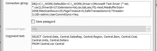
Figure 7-2. Connection string and command text
- At the beginning of the connection string is the location of the current connection's file and the default directory, which you can edit if the new file is in a different folder:
DBQ=C:\_WORK;DefaultDir=C:\_WORK;
- In the command text, change the file name references to the new file name. For example, change Central to South. If you want all the fields from the source file, use the asterisk, instead of listing the fields individually:
SELECT South.* FROM South.csv South
- Click OK, to close the Connection Properties dialog box.
Create a New Connection
The other option is to create a new connection, and use it as the pivot table's data source. The long list of steps may look daunting, but the entire process should only take a couple of minutes:
- Select an empty cell in the workbook that contains the pivot table.
- On the Ribbon's Data tab, in the Get External Data group, click From Other Sources, and then click From Microsoft Query. Depending on your security settings, you may see a security warning.
- In the Choose Data Source dialog box, on the Databases tab, select <New Data Source>, and then click OK.
- Name the data source, such as MyCSV_New, and from the drop-down list of drivers, select Microsoft Text Driver (*.txt,*.csv).
- Click Connect, and leave the check mark for Use Current Directory, because you want to connect to the South.csv file in the C:\_Work directory.
- To connect to a file in a different directory, remove the check mark, click Select Directory, select a different directory, and then click OK.
- Click OK, to close the ODBC Text Setup dialog box.
- For the default table, select the South.csv file, and then click OK, twice.
- In the Query Wizard, select the South.csv file as the table, and then click the arrow button to move all its fields into the query.
- Click Next, three times, to reach the last step in the Query Wizard, and then click Finish.
- In the Import Data dialog box, select PivotTable Report, and select a location for this temporary pivot table, and then click OK.
- Delete the temporary pivot table, which isn't needed now that the connection is established.
- Select a cell in the original pivot table, and on the Ribbon's Options tab, click Change Data Source, and then click Choose Connection.
- Select the new connection, Query from MyCSV_New, in the list, click Open, and then click OK.
Note After you delete the temporary pivot table, you must use the new connection before closing the file, or the connection is automatically deleted.
7.9. Refreshing When a File Opens
Problem
Your pivot table is based on a csv file that is updated every evening, and you want to ensure the pivot table is updated as soon as the file that contains the pivot table opens. This problem is based on the PivotCSV.xlsx sample file.
Solution
You can set a pivot table option to refresh the pivot table automatically, as the file opens. This setting can be used for pivot tables with an external data source, and for pivot tables based on data in the same Excel file as the pivot table.
- Right-click a cell in the pivot table, and then click PivotTable Options.
- On the Data tab, add a check mark to Refresh Data When Opening the File.
- Click OK to close the PivotTable Options dialog box.
7.10. Preventing a Refresh When a File Opens
Problem
In the Trust Center, you have enabled all data connections, and your pivot table is set to refresh when the file opens. This works well, and ensures that the pivot table is automatically updated each morning, when you open the workbook. However, you occasionally want to open the file without having the pivot table refresh, so you can review the previous day's data before moving forward. This problem is based on the Refresh.xlsx sample workbook.
Workaround
Although you can't override the Refresh Data When Opening the File setting, you can undo the refresh, after the file has opened, and before you perform any other tasks.
Click the arrow on the Undo button, on the Quick Access Toolbar, and then click to undo any of the listed PivotTable Refresh actions (see Figure 7-3).
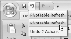
Figure 7-3. Undo PivotTable Refresh
Tip To stop a long refresh in progress, press the Esc key as the file opens.
7.11. Refreshing Every 30 Minutes
Problem
The database to which your pivot table is connected is updated frequently throughout the day, and you would like the pivot table to refresh automatically every 30 minutes. However, when you right-click the pivot table and choose PivotTable Options, you only see an option to Refresh Data When Opening the File. This problem is based on the Shipments.xlsx sample workbook.
Solution
The Refresh Every n Minutes option is in the Connection Properties dialog box. To change the setting, follow these steps:
- Select a cell in the pivot table, and then on the Ribbon's Data tab, in the Connections group, click Properties.
- On the Usage tab, add a check mark to Refresh Every 60 Minutes.
- Change the number of minutes to 30, and then click OK.
Note This option is only available for pivot tables with an external data source. For pivot tables based on an Excel Table in the same workbook, you can use programming to automatically refresh the pivot table when the source data changes, as described in Chapter 11.
7.12. Refreshing All Pivot Tables in a Workbook
Problem
Several pivot tables are in your workbook, based on different Excel Tables. You want to refresh all of them at the same time, instead of refreshing each pivot table individually. This can save you several minutes each day, if you don't have to go to each worksheet and update the pivot tables one at a time. This problem is based on the Sales07.xlsx sample workbook.
Solution
To refresh all the pivot tables in the active workbook at the same time, on the Ribbon's Data tab, in the Connections group, click the upper section of the Refresh All command (see Figure 7-4).
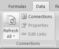
Figure 7-4. Refresh All command
Note Using the Refresh All command also refreshes all external data ranges in the active workbook, and it affects both visible and hidden worksheets.
7.13. Stopping a Refresh in Progress
Problem
You clicked the Refresh button to update your pivot table. The refresh is taking a long time to run, and you want to stop it, so you can work on something else in the workbook, and then run the refresh later. This problem is based on the Shipments.xlsx sample workbook.
Solution
To stop a long refresh, press the Esc key on the keyboard.
If a refresh is running as a background query, you can double-click the Refresh indicator on the status bar (see Figure 7-5). In the External Data Refresh Status dialog box, click the Stop Refresh button, and then close the dialog box.
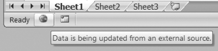
Figure 7-5. Refresh indicator on the status bar
Note When you refresh the pivot table, the entire pivot table is affected. You can't refresh only part of a pivot table, or just add the new data to the pivot cache.
7.14. Creating an OLAP-Based Pivot Table Causes Client Safety Options Error Message
Problem
When you try to create an OLAP-based pivot table, you get the error message "Client Safety options do not allow pass through statements to be issued to the data source." There is no sample file for this problem, but you may encounter this error as you work with your own files.
Solution
This error occurs if you have an OLAP cube in which you opted to rebuild the cube every time the report is opened. To stop the message from appearing when the file opens, you can add a new setting to the Windows Registry.
The steps for this are outlined in the Microsoft Knowledge Base article "You Receive an Error When You Create an OLAP Cube-Based PivotTable in Excel," at http://support.microsoft.com/default.aspx?id=887297.
Caution If you decide to modify the Windows Registry, as described in the Knowledge Base article, follow the instructions carefully, and observe the warnings to back up the Registry before changing it, as well as the security cautions.
7.15. Refreshing a Pivot Table on a Protected Sheet
Problem
You protected the worksheet that contains your pivot table, and under the Allow All Users of This Worksheet To list, you added a check mark to Use Pivot Table Reports. However, when you right-click a cell in the pivot table, the Refresh command is disabled, and you can't refresh the pivot table. This problem is based on the Protect.xlsx sample workbook.
Solution
The worksheet must be unprotected before you can refresh the pivot table. You can do this manually or use programming to unprotect the sheet, refresh the pivot table, and then protect the sheet. A programming example is in Chapter 11.
Note If pivot tables on different sheets use the same pivot cache, the worksheets for all the related pivot tables must be unprotected before any of the pivot tables can be refreshed.
7.16. Refreshing When Two Tables Overlap
Problem
You have two pivot tables on the same worksheet, and sometimes when you modify one of the pivot tables, you get an error message "A PivotTable report cannot overlap another PivotTable report." You want to view them side by side, but would like the second pivot table to move to the right if necessary, instead of creating the error message. This problem is based on the Overlap.xlsx sample workbook.
Workaround
If the pivot table being modified will expand, and if it needs space that's occupied by the other pivot table, you'll see that message. There's no setting you can change that will move the other pivot table, to accommodate the first pivot table.
You could store each pivot table on a separate worksheet, and use multiple windows in the workbook to view them simultaneously:
- To create a new window in the active workbook, on the Ribbon's View tab, in the Window group, click New Window. The title bar shows a number at the end of the file name, to indicate which window is active.
- To view both windows simultaneously, on the Ribbon's View tab, in the Window group, click Arrange All.
- Select Tiled, and add a check mark to Windows of Active Workbook, and then click OK.
- In each window, activate one of the worksheets that contain a pivot table. With this arrangement you can see the pivot tables side by side, but they won't overlap if one of the pivot tables is modified.
7.17. Refreshing Pivot Tables After Queries Have Been Executed
Problem
When you use the Refresh All command on the Ribbon's Data tab, your pivot tables are refreshed before your queries for external data have run. You want to pause the pivot cache refresh until after the queries are executed, to ensure all the current data is displayed in the pivot table. This problem is based on the Refresh.xlsx sample workbook.
You can change a setting for the external data range's connection:
- On the Ribbon's Data tab, click Connections.
- In the list of connections, select the one you want to change, and then click Properties.
- On the Usage tab, remove the check mark from Enable Background Refresh, click OK, and then click Close.
With the Enable Background Refresh option off, other processes will wait while Excel refreshes the query for the external data source.
7.18. Refreshing Pivot Tables: Defer Layout Update
Problem
You frequently make changes to the pivot table layout, moving several of the fields to a different area, and then adding and removing fields from the layout. The pivot table updates after each change, and this slows things down. You'd prefer to make all the changes, and then update the pivot table. This problem is based on the Sales07.xlsx sample workbook.
Solution
To prevent the updates from occurring as you make the changes, you can change a setting in the PivotTable Field List:
- Select a cell in the pivot table.
- In the PivotTable Field List, add a check mark to Defer Layout Update.
- Make the layout changes to the pivot table, and then click Update (see Figure 7-6).

Figure 7-6. Defer Layout Update option and Update button
- When you finish changing the layout and updating the pivot table, remove the check mark from Defer Layout Update.
Note While the Defer Layout Update option is checked, some features of the pivot table, such as Row Labels filters, are disabled.