Chapter 31: Making Your Worksheets
Error Free
In This Chapter
Identify and correcting common formula errors
Using Excel auditing tools
Using formula AutoCorrect
Tracing cell relationships
Checking spelling and related features
It goes without saying that you want your Excel worksheets to produce accurate results. Unfortunately, it's not always easy to be certain that the results are correct — especially if you deal with large, complex worksheets. This chapter introduces the tools and techniques available to help identify, correct, and prevent errors.
Finding and Correcting Formula Errors
Making a change in a worksheet — even a relatively minor change — may produce a ripple effect that introduces errors in other cells. For example, accidentally entering a value into a cell that previously held a formula is all too easy to do. This simple error can have a major impact on other formulas, and you may not discover the problem until long after you make the change — or you may never discover the problem.
Formula errors tend to fall into one of the following general categories:
• Syntax errors: You have a problem with the syntax of a formula. For example, a formula may have mismatched parentheses, or a function may not have the correct number of arguments.
• Logical errors: A formula doesn't return an error, but it contains a logical flaw that causes it to return an incorrect result.
• Incorrect reference errors: The logic of the formula is correct, but the formula uses an incorrect cell reference. As a simple example, the range reference in a Sum formula may not include all the data that you want to sum.
• Semantic errors: An example is a function name that is spelled incorrectly. Excel will attempt to interpret it as a name and will display the #NAME? error.
• Circular references: A circular reference occurs when a formula refers to its own cell, either directly or indirectly. Circular references are useful in a few cases, but most of the time, a circular reference indicates a problem.
• Array formula entry error: When entering (or editing) an array formula, you must press Ctrl+Shift+Enter to enter the formula. If you fail to do so, Excel doesn't recognize the formula as an array formula, and you may get an error or incorrect results.
![]() Refer to Chapter 17 for an introduction to array formulas.
Refer to Chapter 17 for an introduction to array formulas.
• Incomplete calculation errors: The formulas simply aren't calculated fully. To ensure that your formulas are fully calculated, press Ctrl+Alt+Shift+F9.
Syntax errors are usually the easiest to identify and correct. In most cases, you'll know when your formula contains a syntax error. For example, Excel won't permit you to enter a formula with mismatched parentheses. Other syntax errors also usually result in an error display in the cell.
The following sections describe common formula problems and offers advice on identifying and correcting them.
Mismatched parentheses
In a formula, every left parenthesis must have a corresponding right parenthesis. If your formula has mismatched parentheses, Excel usually won't permit you to enter it. An exception to this rule involves a simple formula that uses a function. For example, if you enter the following formula (which is missing a closing parenthesis), Excel accepts the formula and provides the missing parenthesis.
=SUM(A1:A500
A formula may have an equal number of left and right parentheses, but the parentheses may not match properly. For example, consider the following formula, which converts a text string such that the first character is uppercase and the remaining characters are lowercase. This formula has five pairs of parentheses, and they match properly.
=UPPER(LEFT(A1))&RIGHT(LOWER(A1),LEN(A1)-1)
The following formula also has five pairs of parentheses, but they're mismatched. The result displays a syntactically correct formula that simply returns the wrong result.
=UPPER(LEFT(A1)&RIGHT(LOWER(A1),LEN(A1)-1))
Often, parentheses that are in the wrong location will result in a syntax error, which is usually a message that tells you that you entered too many or too few arguments for a function.
Using Formula AutoCorrect
When you enter a formula that has a syntax error, Excel attempts to determine the problem and offers a suggested correction. The accompanying figure shows an example of a proposed correction.
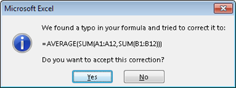
Be careful when accepting corrections for your formulas from Excel because it doesn't always guess correctly. For example, I entered the following formula (which has mismatched parentheses):
=AVERAGE(SUM(A1:A12,SUM(B1:B12))
Excel then proposed the following correction to the formula:
=AVERAGE(SUM(A1:A12,SUM(B1:B12)))
You may be tempted to accept the suggestion without even thinking. In this case, the proposed formula is syntactically correct — but not what I intended. The correct formula is
=AVERAGE(SUM(A1:A12),SUM(B1:B12))
Tip
Excel can help you out with mismatched parentheses. When you're editing a formula and you move the cursor over a parenthesis, Excel displays it (and its matching parenthesis) in bold for about one-half second. In addition, Excel color-codes pairs of nested parentheses while you're editing a formula.
Cells are filled with hash marks
A cell is filled with a series of hash marks (#) for one of two reasons:
• The column is not wide enough to accommodate the formatted numeric value. To correct it, you can make the column wider or use a different number format (see Chapter 25).
• The cell contains a formula that returns an invalid date or time. For example, Excel doesn't support dates prior to 1900 or the use of negative time values. A formula that returns either of these values results in a cell filled with hash marks. Widening the column won't fix it.
Blank cells are not blank
Some Excel users have discovered that by pressing the spacebar, the contents of a cell seem to erase. Actually, pressing the spacebar inserts an invisible space character, which isn't the same as erasing the cell.
For example, the following formula returns the number of nonempty cells in range A1:A10. If you “erase” any of these cells by using the spacebar, these cells are included in the count, and the formula returns an incorrect result.
=COUNTA(A1:A10)
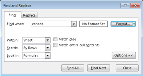
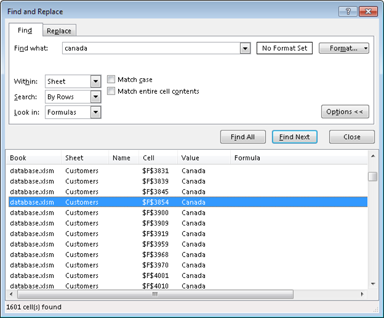
If your formula doesn't ignore blank cells the way that it should, check to make sure that the blank cells are really blank cells. Here's how to search for cells that contain only blank characters:
1. Press Ctrl+F. The Find and Replace dialog box appears.
2. Click the Options button to expand the dialog box so it displays additional options.
3. In the Find What box, enter * *. That's an asterisk, followed by a space, followed by another asterisk.
4. Make sure the Match Entire Cell Contents check box is selected.
5. Click Find All. If any cells that contain only space characters are found, Excel lists the cell address at the bottom of the Find and Replace dialog box.
Extra space characters
If you have formulas or use procedures that rely on comparing text, be careful that your text doesn't contain additional space characters. Adding an extra space character is particularly common when data has been imported from another source.
Excel automatically removes trailing spaces from values that you enter, but trailing spaces in text entries are not deleted. It's impossible to tell just by looking at a cell whether it contains one or more trailing space characters.
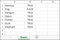
The TRIM function removes leading spaces, trailing spaces, and multiple spaces within a text string. Figure 31.1 shows some text in column A. The formula in B1, which was copied down the column is
=TRIM(A1)=A1
This formula returns FALSE if the text in column A contains leading spaces, trailing spaces, or multiple spaces. In this case, the word Dog in cell A2 contains a trailing space.
Tracing Error Values
Often, an error in one cell is the result of an error in a precedent cell. For help in identifying the cell causing an error value to appear, activate the cell that contains the error and then choose Formulas ⇒ Formula Auditing ⇒ Error Checking ⇒ Trace Error. Excel draws arrows to indicate which cell is the source of the error.
After you identify the error, choose Formulas ⇒ Formula Auditing ⇒ Remove Arrows to get rid of the arrow display.
Figure 31.1
Using a formula to identify cells that contain extra space characters.
Formulas returning an error
A formula may return any of the following error values:
• #DIV/0!
• #N/A
• #NAME?
• #NULL!
• #NUM!
• #REF!
• #VALUE!
The following sections summarize possible problems that may cause these errors.
Tip
Excel allows you to choose how error values are printed. To access this feature, display the Page Setup dialog box and select the Sheet tab. You can choose to print error values as displayed (the default), or as blank cells, dashes, or #N/A. To display the Page Setup dialog box, click the dialog box launcher of the Page Layout ⇒ Page Setup group.
#DIV/0! errors
Division by zero is not a valid operation. If you create a formula that attempts to divide by zero, Excel displays its familiar #DIV/0! error value.
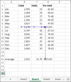
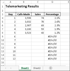
Because Excel considers a blank cell to be zero, you also get this error if your formula divides by a missing value. This problem is common when you create formulas for data that you haven't entered yet, as shown in Figure 31.2. The formula in cell D4, which was copied to the cells below it, is
=C4/B4
This formula calculates the ratio of the values in columns C and B. Data isn't available for all days, so the formula returns a #DIV/0! error.
To avoid the error display, you can use an IF function to check for a blank cell in column B:
=IF(B4=0,””,C4/B4)
This formula displays an empty string if cell B4 is blank or contains 0; otherwise, it displays the calculated value.
Figure 31.2
#DIV/0! errors occur when the data in column B is missing.
Another approach is to use an IFERROR function to check for any error condition. The following formula, for example, displays an empty string if the formula results in any type of error:
=IFERROR(C4/B4,””)
Note
The IFERROR function was introduced in Excel 2007. For compatibility with previous versions of Excel, use this formula:
=IF(ISERROR(C4/B4),””,C4/B4)
#N/A errors
The #N/A error occurs if any cell referenced by a formula displays #N/A.
Note
Some users like to use =NA() or #N/A explicitly for missing data. This method makes it perfectly clear that the data is not available and hasn't been deleted accidentally.
The #N/A error also occurs when a LOOKUP function (HLOOKUP, LOOKUP, MATCH, or VLOOKUP) can't find a match.
If you would like to display an empty string instead of #N/A use the IFNA function in a formula like this:
=IFNA(VLOOKUP(A1,C1:F50,4,FALSE),””)
Note
The IFNA function is new to Excel 2013. For compatibility with previous versions use a formula like this:
=IF(ISNA(VLOOKUP(A1,C1:F50,4,FALSE)),””,VLOOKUP(A1,C1:F50,4,FALSE))
#NAME? errors
The #NAME? error occurs under these conditions:
• The formula contains an undefined range or cell name.
• The formula contains text that Excel interprets as an undefined name. A misspelled function name, for example, generates a #NAME? error.
• The formula contains text that isn't enclosed in quotation marks.
• The formula contains a range reference that omits the colon between the cell addresses.
• The formula uses a worksheet function that's defined in an add-in, and the add-in is not installed.
Caution
Excel has a bit of a problem with range names. If you delete a name for a cell or range and the name is used in a formula, the formula continues to use the name, even though it's no longer defined. As a result, the formula displays #NAME?. You might expect Excel to automatically convert the names to their corresponding cell references, but this doesn't happen.
#NULL! errors
A #NULL! error occurs when a formula attempts to use an intersection of two ranges that don't actually intersect. Excel's intersection operator is a space. The following formula, for example, returns #NULL! because the two ranges don't intersect:
=SUM(B5:B14 A16:F16)
The following formula doesn't return #NULL! but displays the contents of cell B9, which represents the intersection of the two ranges:
=SUM(B5:B14 A9:F9)
You also see a #NULL! error if you accidentally omit an operator in a formula. For example, this formula is missing the second operator:
= A1+A2 A3
#NUM! errors
A formula returns a #NUM! error if any of the following occurs:
• You pass a nonnumeric argument to a function when a numeric argument is expected (for example, $1,000 instead of 1000).
• You pass an invalid argument to a function. For example, this formula returns #NUM!:
=SQRT(-12)
• A function that uses iteration can't calculate a result. Examples of functions that use iteration are IRR and RATE.
• A formula returns a value that is too large or too small. Excel supports values between –1E-307 and 1E+307.
#REF! errors
A #REF! error occurs when a formula uses an invalid cell reference. This error can occur in the following situations:
• You delete the row column of a cell that is referenced by the formula. For example, the following formula displays a #REF! error if row 1, column A, or column B is deleted:
=A1/B1
• You delete the worksheet of a cell that is referenced by the formula. For example, the following formula displays a #REF! error if Sheet2 is deleted:
=Sheet2!A1
• You copy a formula to a location that invalidates the relative cell references. For example, if you copy the following formula from cell A2 to cell A1, the formula returns #REF! because it attempts to refer to a nonexistent cell.
=A1-1
• You cut a cell (choose Home ⇒ Clipboard ⇒ Cut) and then paste it to a cell that's referenced by a formula. The formula will display #REF!.
#VALUE! errors
A #VALUE! error is very common and can occur under the following conditions:
• An argument for a function is of an incorrect data type, or the formula attempts to perform an operation using incorrect data. For example, a formula that adds a value to a text string returns the #VALUE! error.
• A function's argument is a range when it should be a single value.
• A custom worksheet function is not calculated. You can press Ctrl+Alt+F9 to force a recalculation.
• A custom worksheet function attempts to perform an operation that is not valid. For example, custom functions can't modify the Excel environment or make changes to other cells.
• You forget to press Ctrl+Shift+Enter when entering an Array formula.
Absolute/relative reference problems
As I describe in Chapter 10, a cell reference can be relative (for example, A1), absolute (for example, $A$1), or mixed (for example, $A1 or A$1). The type of cell reference that you use in a formula is relevant only if the formula will be copied to other cells.
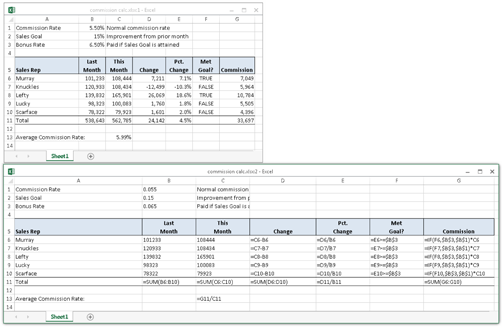
A common problem is using a relative reference when you should use an absolute reference. As shown in Figure 31.3, cell C1 contains a tax rate, which is used in the formulas in column C. The formula in cell C4 is
=B4+(B4*$C$1)
Figure 31.3
Formulas in the range C4:C7 use an absolute reference to cell C1.
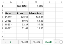
Notice that the reference to cell C1 is an absolute reference. When the formula is copied to other cells in column C, the formula continues to refer to cell C1. If the reference to cell C1 were a relative reference, the copied formulas would return an incorrect result.
Operator precedence problems
As I describe in Chapter 10, Excel has some straightforward rules about the order in which mathematical operations are performed. When in doubt (or when you simply need to clarify your intentions), you should use parentheses to ensure that operations are performed in the correct order. For example, the following formula multiplies A1 by A2 and then adds 1 to the result. The multiplication is performed first because it has a higher order of precedence.
=1+A1*A2
The following is a clearer version of this formula. The parentheses aren't necessary, but in this case, the order of operations is perfectly obvious.
=1+(A1*A2)
Notice that the negation operator symbol is exactly the same as the subtraction operator symbol. This, as you may expect, can cause some confusion. Consider these two formulas:
=-3^2
=0-3^2
The first formula, as expected, returns 9. The second formula, however, returns –9. Squaring a number always produces a positive result, so how is it that Excel can return the –9 result?
In the first formula, the minus sign is a negation operator and has the highest precedence. However, in the second formula, the minus sign is a subtraction operator, which has a lower precedence than the exponentiation operator. Therefore, the value 3 is squared, and then the result is subtracted from 0 (zero), which produces a negative result.
Using parentheses, as shown in the following formula, causes Excel to interpret the operator as a minus sign rather than a negation operator. This formula returns –9.
=-(3^2)
Formulas are not calculated
If you use custom worksheet functions written in VBA, you may find that formulas that use these functions fail to get recalculated and may display incorrect results. For example, assume that you wrote a VBA function that returns the number format of a referenced cell. If you change the number format, the function will continue to display the previous number format. That's because changing a number format doesn't trigger a recalculation.
To force a single formula to be recalculated, select the cell, press F2, and then press Enter. To force a recalculation of all formulas, press Ctrl+Alt+F9.
Actual versus displayed values
You may encounter a situation in which values in a range don't appear to add up properly. For example, Figure 31.4 shows a worksheet with the following formula entered into each cell in the range B2:B4:
=1/3
Figure 31.4
A simple demonstration of numbers that appear to add up incorrectly.
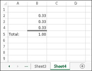
Cell B5 contains the following formula:
=SUM(B2:B4)
All the cells are formatted to display with three decimal places. As you can see, the formula in cell B5 appears to display an incorrect result. (You may expect it to display 0.99.) The formula, of course, does return the correct result. The formula uses the actual values in the range B2:B4 not the displayed values.
You can instruct Excel to use the displayed values by selecting the Set Precision as Displayed check box of the Advanced section of the Excel Options dialog box. (Choose File ⇒ Options to display this dialog box.)
Caution
Be very careful with the Set Precision as Displayed option. This option also affects normal values (nonformulas) that have been entered into cells. For example, if a cell contains the value 4.68 and is displayed with no decimal places (that is, 5), selecting the Precision as Displayed check box converts 4.68 to 5.00. This change is permanent, and you can't restore the original value if you later clear the Set Precision as Displayed check box. A better approach is to use the ROUND function to round off the values to the desired number of decimal places.
Floating point number errors
Computers, by their very nature, don't have infinite precision. Excel stores numbers in binary format by using 8 bytes, which can handle numbers with 15-digit accuracy. Some numbers can't be expressed precisely by using 8 bytes, so the number is stored as an approximation.
To demonstrate how this lack of precision may cause problems, enter the following formula into cell A1:
=(5.1-5.2)+1
The result should be 0.9. However, if you format the cell to display 15 decimal places, you discover that Excel calculates the formula with a result of 0.899999999999999. This result occurs because the operation in parentheses is performed first, and this intermediate result stores in binary format by using an approximation. The formula then adds 1 to this value, and the approximation error is propagated to the final result.
In many cases, this type of error doesn't present a problem. However, if you need to test the result of that formula by using a logical operator, it may present a problem. For example, the following formula (which assumes that the previous formula is in cell A1) returns FALSE:
=A1=.9
One solution to this type of error is to use the ROUND function. The following formula, for example, returns TRUE because the comparison is made by using the value in A1 rounded to one decimal place.
=ROUND(A1,1)=0.9
Here's another example of a “precision” problem. Try entering the following formula:
=(1.333-1.233)-(1.334-1.234)
This formula should return 0, but it actually returns –2.220446E-16 (a number very close to zero).
If that formula is in cell A1, the following formula returns Not Zero.
=IF(A1=0,”Zero”,”Not Zero”)
One way to handle these “very close to zero” rounding errors is to use a formula like this:
=IF(ABS(A1)<1E-6,”Zero”,”Not Zero”)
This formula uses the less-than operator (<) to compare the absolute value of the number with a very small number. This formula returns Zero.
“Phantom link” errors
You may open a workbook and see a message like the one shown in Figure 31.5. This message sometimes appears even when a workbook contains no linked formulas. Often, these phantom links are created when you copy a worksheet that contains names.
Figure 31.5
Excel's way of asking whether you want to update links in a workbook.
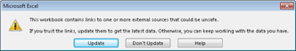
First, try choosing File ⇒ Info ⇒ Edit Links to Files to display the Edit Links dialog box. Then select each link and click Break Link. If that doesn't solve the problem, this phantom link may be caused by an erroneous name. Choose Formulas ⇒ Defined Names ⇒ Name Manager and scroll through the list of names in the Name Manager dialog box. If you see a name that refers to #REF!, delete the name. The Name Manager dialog box has a Filter button that lets you filter the names. For example, you can filter the lists to display only the names with errors.
Using Excel Auditing Tools
Excel includes a number of tools that can help you track down formula errors. This section describes the auditing tools built in to Excel.
Identifying cells of a particular type
The Go to Special dialog box (shown in Figure 31.6) is a handy tool that enables you to locate cells of a particular type. To display this dialog box, choose Home ⇒ Editing ⇒ Find & Select ⇒ Go to Special.
Figure 31.6
The Go to Special dialog box.
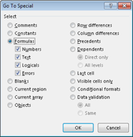
Note
If you select a multicell range before displaying the Go to Special dialog box, the command operates only within the selected cells. If a single cell is selected, the command operates on the entire worksheet.
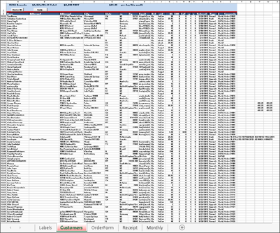
You can use the Go to Special dialog box to select cells of a certain type, which can often help you identify errors. For example, if you choose the Formulas option, Excel selects all the cells that contain a formula. If you zoom the worksheet out to a small size, you can get a good idea of the worksheet's organization (see Figure 31.7). To zoom a worksheet, use the zoom controls on the right side of the status bar or press Ctrl while you move the scroll wheel on your mouse.
Figure 31.7
Zooming out and selecting all formula cells can give you a good overview of how the worksheet is designed.
Tip
Selecting the formula cells may also help you spot a common error: namely, a formula that has been replaced accidentally with a value. If you find a cell that's not selected amid a group of selected formula cells, chances are good that the cell previously contained a formula that has been replaced by a value.
Viewing formulas
You can become familiar with an unfamiliar workbook by displaying the formulas rather than the results of the formulas. To toggle the display of formulas, choose Formulas ⇒ Formula Auditing ⇒ Show Formulas. You may want to create a second window for the workbook before issuing this command. This way, you can see the formulas in one window and the results of the formula in the other window. Choose View ⇒ Window ⇒ New Window to open a new window.
Using the Inquire Add-in
Some versions of Excel 2013 include a useful auditing add-in called Inquire. To install Inquire, follow these steps:
1. Choose File ⇒ Options. The Excel Options dialog box appears.
2. Select the Add-ins tab.
3. At the bottom of the dialog box, choose COM Add-ins from the Manage drop-down list, and click Go. The COM Add-Ins dialog box appears.
4. Place a check mark next to Inquire Add-in and click OK. The add-in will be loaded automatically when Excel starts.
Note: If Inquire is not listed, that means your version of Excel does not include the add-in.
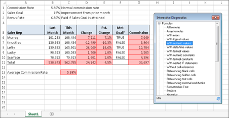
Inquire is accessible from the Inquire tab on the Ribbon. You can use this add-in to
• Compare versions of a workbook
• Analyze a workbook for potential problem and inconsistencies
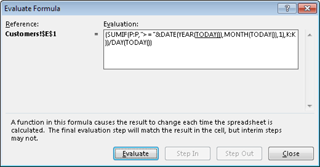
• Display interactive diagnostics (shown here)
• Visualize links between workbook and worksheets
• Clear excess cell formatting
• Manage passwords
Tip
You can also press Ctrl+` (the accent grave key, typically located above the Tab key) to toggle between Formula view and Normal view.
Figure 31.8 shows an example of a worksheet displayed in two windows. The window on the top shows Normal view (formula results), and the window on the bottom displays the formulas. Choosing View ⇒ Window ⇒ View Side by Side, which allows synchronized scrolling, is also useful for viewing two windows.
Figure 31.8
Displaying formulas (bottom window) and their results (top window).
![]() See Chapter 4 for more information about this command.
See Chapter 4 for more information about this command.
Tracing cell relationships
To understand how to trace cell relationships, you need to familiarize yourself with the following two concepts:
• Cell precedents: Applicable only to cells that contain a formula, a formula cell's precedents are all the cells that contribute to the formula's result. A direct precedent is a cell that you use directly in the formula. An indirect precedent is a cell that isn't used directly in the formula but is used by a cell that you refer to in the formula.
• Cell dependents: These formula cells depend upon a particular cell. A cell's dependents consist of all formula cells that use the cell. Again, the formula cell can be a direct dependent or an indirect dependent.
For example, consider this simple formula entered into cell A4:
=SUM(A1:A3)
Cell A4 has three precedent cells (A1, A2, and A3), which are all direct precedents. Cells A1, A2, and A3 all have at least one dependent cell (cell A4), and they're all direct dependents.
Identifying cell precedents for a formula cell often sheds light on why the formula isn't working correctly. Conversely, knowing which formula cells depend on a particular cell is also helpful. For example, if you're about to delete a formula, you may want to check whether it has any dependents.
Identifying precedents
You can identify cells used by a formula in the active cell in a number of ways:
• Press F2. The cells that are used directly by the formula are outlined in color, and the color corresponds to the cell reference in the formula. This technique is limited to identifying cells on the same sheet as the formula.
• Choose Home ⇒ Editing ⇒ Find & Select ⇒ Go to Special to display the Go to Special dialog box. Select the Precedents option and then select either Direct Only (for direct precedents only) or All Levels (for direct and indirect precedents). Click OK, and Excel selects the precedent cells for the formula. This technique is limited to identifying cells on the same sheet as the formula.
• Press Ctrl+[. This selects all direct precedent cells on the active sheet.
• Press Ctrl+Shift+{. This selects all precedent cells (direct and indirect) on the active sheet.
• Choose Formulas ⇒ Formula Auditing ⇒ Trace Precedents. Excel will draw arrows to indicate the cell's precedents. Click this button multiple times to see additional levels of precedents. Choose Formulas ⇒ Formula Auditing ⇒ Remove Arrows to hide the arrows. Figure 31.9 shows a worksheet with precedent arrows drawn to indicate the precedents for the formula in cell C13.
Identifying dependents
You can identify formula cells that use a particular cell in a number of ways:
• Choose Home ⇒ Editing ⇒ Find & Select ⇒ Go to Special to display the Go to Special dialog box. Select the Dependents option and then select either Direct Only (for direct dependents only) or All Levels (for direct and indirect dependents). Click OK. Excel selects the cells that depend upon the active cell. This technique is limited to identifying cells on the active sheet only.
• Press Ctrl+]. This selects all direct dependent cells on the active sheet.
• Press Ctrl+Shift+}. This selects all dependent cells (direct and indirect) on the active sheet.
• Choose Formulas ⇒ Formula Auditing ⇒ Trace Dependents. Excel will draw arrows to indicate the cell's dependents. Click this button multiple times to see additional levels of dependents. Choose Formulas ⇒ Formula Auditing ⇒ Remove Arrows to hide the arrows.
Figure 31.9
This worksheet displays arrows that indicate cell precedents for the formula in cell C13.
Tracing error values
If a formula displays an error value, Excel can help you identify the cell that is causing that error value. An error in one cell is often the result of an error in a precedent cell. Activate a cell that contains an error value and then choose Formulas ⇒ Formula Auditing ⇒ Error Checking ⇒ Trace Error. Excel draws arrows to indicate the error source.
Fixing circular reference errors
If you accidentally create a circular reference formula, Excel displays a warning message — Circular Reference — with the cell address, in the status bar, and also draws arrows on the worksheet to help you identify the problem. If you can't figure out the source of the problem, choose Formulas ⇒ Formula Auditing ⇒ Error Checking ⇒ Circular References. This command displays a list of all cells that are involved in the circular references. Start by selecting the first cell listed and then work your way down the list until you figure out the problem.
Using the background error-checking feature
Some people may find it helpful to take advantage of the Excel automatic error-checking feature. This feature is enabled or disabled via the Enable Background Error Checking check box, found on the Formulas tab of the Excel Options dialog box, shown in Figure 31.10. In addition, you can use the check boxes in the Error Checking Rules section to specify which types of errors to check.
Figure 31.10
Excel can check your formulas for potential errors.
When error checking is turned on, Excel continually evaluates the formulas in your worksheet. If a potential error is identified, Excel places a small triangle in the upper-left corner of the cell. When the cell is activated, a drop-down control appears. Clicking this drop-down control provides you with options. Figure 31.11 shows the options that appear when you click the drop-down control in a cell that contains a #DIV/0! error. The options vary, depending on the type of error.
Figure 31.11
After you click an error, drop-down control gives you a list of options.
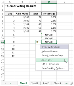
In many cases, you'll choose to ignore an error by selecting the Ignore Error option. Selecting this option eliminates the cell from subsequent error checks. However, all previously ignored errors can be reset so that they appear again. (Use the Reset Ignored Errors button on the Formulas tab of the Excel Options dialog box.)
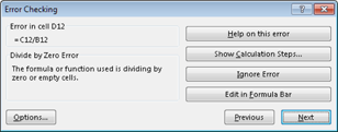
You can choose Formulas ⇒ Formula Auditing ⇒ Error Checking to display a dialog box that describes each potential error cell in sequence, much like using a spell-checking command. This command is available even if you disable background error checking. Figure 31.12 shows the Error Checking dialog box. This dialog box is modeless: that is, you can still access your worksheet when the Error Checking dialog box is displayed.
Figure 31.12
Use the Error Checking dialog box to cycle through potential errors identified by Excel.
Caution
The error-checking feature isn't perfect. In fact, it's not even close to perfect. In other words, you can't assume that you have an error-free worksheet simply because Excel doesn't identify any potential errors! Also, be aware that this error-checking feature won't catch a very common type of error: namely, overwriting a formula cell with a value.