
4. Creating Advanced Formulas
In This Chapter
Using Iteration and Circular References
Applying Data-Validation Rules to Cells
Using Dialog Box Controls on a Worksheet
Excel is a versatile program with many uses, from acting as a checkbook to a flat-file database-management system, to an equation solver, to a glorified calculator. For most business users, however, Excel’s forte is building models that enable quantification of particular aspects of the business. The skeleton of the business model is made up of the chunks of data entered, imported, or copied into the worksheets. But the lifeblood of the model and the animating force behind it is the collection of formulas for summarizing data, answering questions, and making predictions.
You saw in Chapter 3, “Building Basic Formulas,” that, armed with the humble equal sign and Excel’s operators and operands, you can cobble together useful, robust formulas. But Excel has many other tricks up its digital sleeve, and these techniques enable you to create muscular formulas that can take your business models to the next level.
Working with Arrays
When you work with a range of cells, it might appear as though you’re working with a single thing. In reality, however, Excel treats the range as a number of discrete units.
This is in contrast with the subject of this section: the array. An array is a group of cells or values that Excel treats as a unit. In a range configured as an array, for example, Excel no longer treats the cells individually. Instead, it works with all the cells at once, which means you can apply a formula to every cell in the range by using just a single operation, for example.
You create arrays either by running a function that returns an array result (such as DOCUMENTS(); see the section “Functions That Use or Return Arrays,” later in this chapter) or by entering an array formula, which is a single formula that either uses an array as an argument or enters its results in multiple cells.
Using Array Formulas
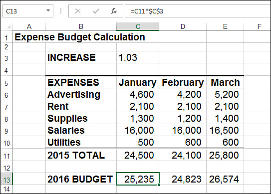
Here’s a straightforward example that illustrates how array formulas work. In the Expenses workbook shown in Figure 4.1, the 2016 BUDGET totals are calculated using a separate formula for each month, as shown here:

Note
You can download this chapter’s sample workbooks at www.mcfedries.com/books/book.php?title=excel-2016-formulas-and-functions.
You can replace all three formulas with a single array formula by following these steps:
1. Select the range you want to use for the array formula. In the 2016 BUDGET example, you’d select C13:E13.
2. Type the formula and, in the places where you would normally enter a cell reference, type a range reference that includes the cells you want to use. Do not—I repeat, do not—press Enter when you’re done. In the example, you’d type =C11:E11*$C$3.
3. To enter the formula as an array, press Ctrl+Shift+Enter.
The 2016 BUDGET cells (C13, D13, and E13) now contain the same formula:
{=C11:E11*$C$3}
In other words, you were able to enter a formula into three different cells by using just a single operation. This saves you tremendous amounts of time when you would otherwise have to enter the same formula into many different cells.
Notice that the formula is surrounded by braces ({ }). This identifies the formula as an array formula. (When you enter array formulas, you never need to enter these braces yourself; Excel adds them automatically when you press Ctrl+Shift+Enter.)
Note
Because Excel treats an array as a unit, you can’t move or delete part of an array. If you need to work with an array, you must select the whole thing. If you want to reduce the size of an array, select it, select the formula bar, and then press Ctrl+Enter to change the entry to a normal formula. You can then select the smaller range and reenter the array formula.
Note that you can select an array quickly by selecting one of its cells and pressing Ctrl+/.
Understanding Array Formulas
To understand how Excel processes an array, you need to keep in mind that Excel always sets up a correspondence between the array cells and the cells of whatever range you entered into the array formula. In the 2016 BUDGET example, the array consists of cells C13, D13, and E13, and the range used in the formula consists of cells C11, D11, and E11. Excel sets up correspondences between array cell C13 and input cell C11, between D13 and D11, and between E13 and E11. To calculate the value of cell C13 (the January 2016 BUDGET), for example, Excel just grabs the input value from cell C11 and substitutes that in the formula. Figure 4.2 shows a diagram of this process.
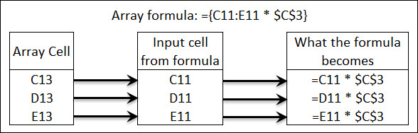
Figure 4.2 When processing an array formula, Excel sets up a correspondence between the array cells and the range used in the formula.
Array formulas can be confusing, but if you keep these correspondences in mind, you should have no trouble figuring out what’s going on.
Array Formulas That Operate on Multiple Ranges
In the preceding example, the array formula operated on a single range, but array formulas also can operate on multiple ranges. For example, consider the Invoice Template worksheet shown in Figure 4.3. The totals in the Extension column (cells F12 through F16) are generated by a series of formulas that multiply the item’s price by the quantity ordered:
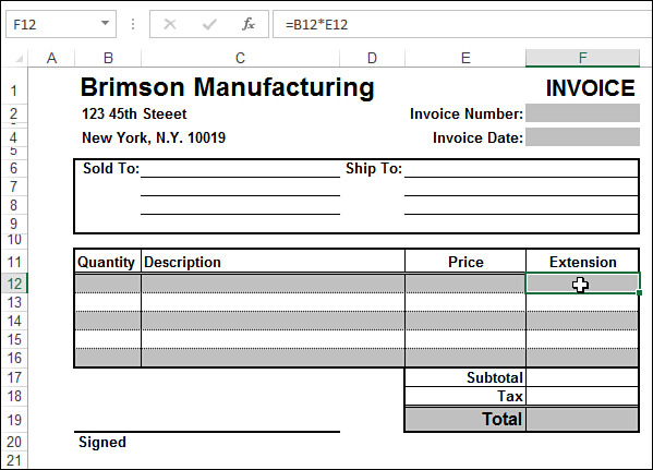

You can replace all these formulas by making the following entry as an array formula into the range F12:F16:
=B12:B16*E12:E16
Again, you’ve created the array formula by replacing each cell reference with the corresponding range (and by pressing Ctrl+Shift+Enter).
You don’t have to enter array formulas in multiple cells. For example, if you don’t need the Extended totals in the Invoice Template worksheet, you can still calculate the Subtotal by making the following entry an array formula in cell F17:
=SUM(B12:B16*E12:E16)
Using Array Constants
In the array formulas you’ve seen so far, the array arguments have been cell ranges. You also can use constant values as array arguments. This procedure enables you to input values into a formula without having them clutter your worksheet.
To enter an array constant in a formula, observe the following guidelines while entering the values right in the formula:
![]() Enclose the values in braces (
Enclose the values in braces ({}).
![]() If you want Excel to treat the values as a row, type a comma after each value (except the last value).
If you want Excel to treat the values as a row, type a comma after each value (except the last value).
![]() If you want Excel to treat the values as a column, type a semicolon after each value (except the last value).
If you want Excel to treat the values as a column, type a semicolon after each value (except the last value).
For example, the following array constant is the equivalent of entering the individual values in a column on your worksheet:
{1;2;3;4}
Similarly, the following array constant is equivalent to entering the values in a worksheet range of three columns and two rows:
{1,2,3;4,5,6}
As a practical example, Figure 4.4 shows two different array formulas. The one on the left (used in the range E4:E7) calculates various loan payments, given the different interest rates in the range C5:C8. The array formula on the right (used in the range F4:F7) does the same thing, but the interest rate values are entered as an array constant directly in the formula.
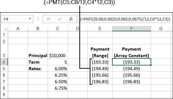
Figure 4.4 Using array constants in your array formulas means you don’t have to clutter your worksheet with the input values.
![]() To learn how the
To learn how the PMT() function works, see “Calculating a Loan Payment,” p. 435.
Functions That Use or Return Arrays
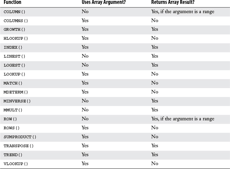
Many of Excel’s worksheet functions either require an array argument or return an array result (or both). Table 4.1 lists several of these functions and explains how each one uses arrays. (See Part II, “Harnessing the Power of Functions,” for explanations of these functions.)
Note
When you use functions that return arrays, be sure to select a range that’s large enough to hold the resulting array and then enter the function as an array formula.
![]() Arrays become truly powerful weapons in your Excel arsenal when you combine them with worksheet functions such as
Arrays become truly powerful weapons in your Excel arsenal when you combine them with worksheet functions such as IF() and SUM(). I’ll provide you with many examples of array formulas as I introduce you to Excel’s worksheet functions throughout Part II. In particular, see “Combining Logical Functions with Arrays,” p. 173.
Using Iteration and Circular References
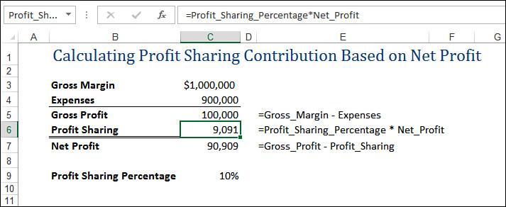
A common business problem involves calculating a profit-sharing plan contribution as a percentage of a company’s net profits. This isn’t a simple multiplication problem because the net profit is determined partly by the profit-sharing figure. For example, suppose that a company has revenue of $1,000,000 and expenses of $900,000, which leaves gross profit of $100,000. The company also sets aside 10% of net profits for profit sharing. The net profit is calculated with the following formula:
Net Profit = Gross Profit - Profit Sharing Contribution
This is called a circular reference formula because there are terms on the left and right sides of the equal sign that depend on each other. Specifically, Profit Sharing Contribution is derived with the following formula:
Profit Sharing Contribution = (Net Profit) * 0.1
![]() Circular references are usually a bad thing to have in a spreadsheet model. To learn how to combat the bad kind, see “Fixing Circular References,” p. 118. (Chapter 5)
Circular references are usually a bad thing to have in a spreadsheet model. To learn how to combat the bad kind, see “Fixing Circular References,” p. 118. (Chapter 5)
One way to solve such a formula is to guess at an answer and see how close you come. For example, because profit sharing should be 10% of net profits, a good first guess might be 10% of gross profits, or $10,000. If you plug this number into the formula, you end up with a net profit of $90,000. However, this isn’t right because 10% of $90,000 is $9,000. Therefore, the profit-sharing guess is off by $1,000.
So, you can try again. This time, use $9,000 as the profit-sharing number. Plugging this new value into the formula gives a net profit of $91,000. This number translates into a profit-sharing contribution of $9,100—which is off by only $100.
If you continue this process, your profit-sharing guesses will get closer to (that is, it will converge on) the calculated value. When the guesses are close enough (for example, within $1), you can stop and pat yourself on the back for finding the solution. This technique is called iteration.
Of course, you didn’t spend your (or your company’s) hard-earned money on a computer so that you could do this sort of thing by hand. Excel makes iterative calculations a breeze, as you see in the following procedure:
1. Set up your worksheet and enter your circular reference formula. Figure 4.5 shows a worksheet for the profit-sharing example just discussed. If Excel displays a dialog box telling you that it can’t resolve circular references, click OK and then select Formulas, Remove Arrows (see Chapter 5).

2. Select File, Options to display the Excel Options dialog box.
3. Click Formulas.
4. Activate the Enable Iterative Calculation check box.
5. Use the Maximum Iterations spin box to specify the number of iterations you need. In most cases, the default figure of 100 is more than enough.
6. Use the Maximum Change text box to tell Excel how accurate you want your results to be. The smaller the number, the longer the iteration takes and the more accurate the calculation will be. Again, the default value of 0.001 is a reasonable compromise in most situations.
7. Click OK. Excel begins the iteration and stops when it has found a solution (see Figure 4.6).
Tip
If you want to watch the progress of the iteration, select the Manual option button in the Calculation Options section of the Formulas tab and enter 1 in the Maximum Iterations spin box. When you return to your worksheet, each time you press F9, Excel performs a single pass of the iteration.
Consolidating Multisheet Data
Many businesses create worksheets for specific tasks and then distribute them to various departments. The most common example is budgeting. Accounting might create a generic “budget” template that each department or division in the company must fill out and return. Similarly, you often see worksheets distributed for inventory requirements, sales forecasting, survey data, experimental results, and more.
Creating these worksheets, distributing them, and filling them in are all straightforward operations. However, the tricky part comes when the sheets are returned to the originating department, and all the new data must be combined into a summary report showing companywide totals. This task is called consolidating the data, and it’s often no picnic, especially for large worksheets. However, as you’ll soon see, Excel has some powerful features that can take the drudgery out of consolidation.
Excel can consolidate your data using one of the following two methods:
![]() Consolidating by position—With this method, Excel consolidates the data from several worksheets, using the same range coordinates on each sheet. You can use this method if the worksheets you’re consolidating have an identical layout.
Consolidating by position—With this method, Excel consolidates the data from several worksheets, using the same range coordinates on each sheet. You can use this method if the worksheets you’re consolidating have an identical layout.
![]() Consolidating by category—This method tells Excel to consolidate the data by looking for identical row and column labels in each sheet. For example, if one worksheet lists monthly Gizmo sales in row 1 and another lists monthly Gizmo sales in row 5, you can consolidate this information as long as both sheets have a “Gizmo” label at the beginning of these rows.
Consolidating by category—This method tells Excel to consolidate the data by looking for identical row and column labels in each sheet. For example, if one worksheet lists monthly Gizmo sales in row 1 and another lists monthly Gizmo sales in row 5, you can consolidate this information as long as both sheets have a “Gizmo” label at the beginning of these rows.
In both cases, you specify one or more source ranges (the ranges that contain the data you want to consolidate) and a destination range (the range where the consolidated data will appear). The next couple of sections take you through the details for both consolidation methods.
Consolidating by Position
If the sheets you’re working with have the same layout, consolidating by position is the easiest way to go. For example, check out the three workbooks—Division I Budget, Division II Budget, and Division III Budget—shown in Figure 4.7. As you can see, each sheet uses the same row and column labels, so they’re perfect candidates for consolidation by position.

Begin by creating a new worksheet that has the same layout as the sheets you’re consolidating. Figure 4.8 shows a new Consolidation workbook that I’ll use to consolidate the three budget sheets.
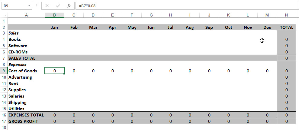
Figure 4.8 When consolidating by position, create a separate consolidation worksheet that uses the same layout as the sheets you’re consolidating.
Let’s look at how to go about consolidating the sales data in the three budget worksheets shown in Figure 4.7. We’re dealing with three source ranges:
'[Division I Budget]Details'!B4:M6
'[Division II Budget]Details'!B4:M6
'[Division III Budget]Details'!B4:M6
With the consolidation sheet active, follow these steps to consolidate by position:
1. Select the upper-left corner of the destination range. In the Consolidate By Position worksheet, the cell to select is B4.
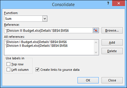
2. Select Data, Consolidate. Excel displays the Consolidate dialog box.
3. In the Function drop-down list, click the operation to use during the consolidation. You’ll use Sum most of the time, but Excel has 10 other operations to choose from, including Count, Average, Max, and Min.
4. In the Reference text box, enter a reference for one of the source ranges. Use one of the following methods:
• Type the range coordinates by hand. If the source range is in another workbook, be sure to include the workbook name enclosed in square brackets. If the workbook is in a different drive or folder, include the full path to the workbook as well.
• If the sheet is open, select it (either by clicking it or by clicking it in the View, Switch Windows menu), and then use your mouse to highlight the range.
• If the workbook isn’t open, click Browse, select the file in the Browse dialog box, and then click OK. Excel adds the workbook path to the Reference box. Fill in the sheet name and the range coordinates.
5. Click Add. Excel adds the range to the All References box (see Figure 4.9).
6. Repeat steps 4 and 5 to add all the source ranges.
7. If you want the consolidated data to change whenever you make changes to the source data, leave the Create Links to Source Data check box selected.
8. Click OK. Excel gathers the data, consolidates it, and then adds it to the destination range (see Figure 4.10).
If you chose not to create links to the source data in step 7, Excel just fills the destination range with the consolidation totals. However, if you did create links, Excel does three things:
![]() Adds link formulas to the destination range for each cell in the source ranges you selected
Adds link formulas to the destination range for each cell in the source ranges you selected
![]() To get the details on link formulas, see “Working with Links in Formulas,” p. 71.
To get the details on link formulas, see “Working with Links in Formulas,” p. 71.
![]() Consolidates the data by adding
Consolidates the data by adding SUM() functions (or whichever operation you selected in the Function list) that total the results of the link formulas
![]() Outlines the consolidation worksheet and hides the link formulas, as you can see in Figure 4.10
Outlines the consolidation worksheet and hides the link formulas, as you can see in Figure 4.10
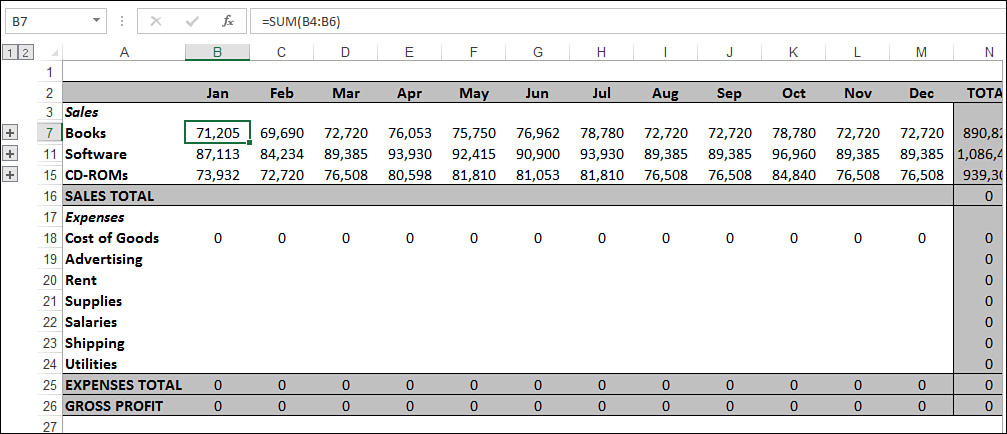
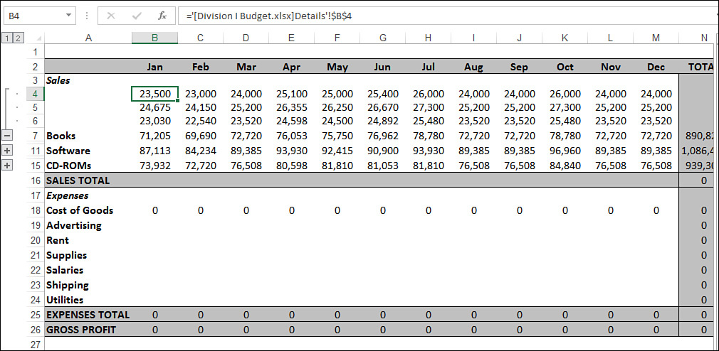
If you display the Level 1 data, you’ll see the linked formulas. For example, Figure 4.11 shows the detail for the consolidated sales number for Books in January (cell B7). Cells B4, B5, and B6 contain formulas that link to the corresponding cells in the three budget worksheets (for example, '[Division I Budget.xlsx]Details'!$B$4).
Consolidating by Category
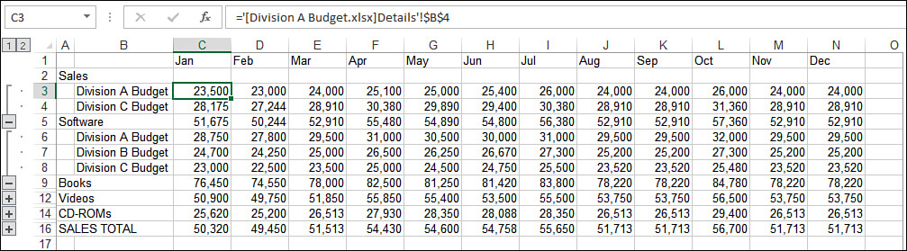
If you want to consolidate date from worksheets that don’t use the same layout, you need to tell Excel to consolidate the data by category. In this case, Excel examines each of your source ranges and consolidates data that uses the same row or column labels. For example, take a look at the Sales rows in the three worksheets shown in Figure 4.12.

As you can see, Division C sells books, software, videos, and CD-ROMs; Division B sells books and CD-ROMs; and Division A sells software, books, and videos. Here’s how you go about consolidating these numbers. (Note that I’m skipping over some of the details given in the preceding section.)
1. Create or select a new worksheet for the consolidation and select the upper-left corner of the destination range. It isn’t necessary to enter labels for the consolidated data because Excel does it for you automatically. However, if you want to see the labels in a particular order, it’s okay to enter them yourself.
Caution
If you enter the labels yourself, make sure that you spell the labels exactly as they’re spelled in the source worksheets.
2. Select Data, Consolidate to display the Consolidate dialog box.
3. In the Function drop-down list, select the operation to use during the consolidation.
4. In the Reference text box, enter a reference for one of the source ranges. In this case, make sure you include in each range the row and column labels for the data.
5. Click Add to add the range to the All References box.
6. Repeat steps 4 and 5 to add all the source ranges.
7. If you want the consolidated data to change whenever you make changes to the source data, leave the Create Links to Source Data check box selected.
8. If you want Excel to use the data labels in the top row of the selected ranges, select the Top Row check box. If you want Excel to use the data labels in the left column of the source ranges, select the Left Column check box.
9. Click OK. Excel gathers the data according to the row and column labels, consolidates it, and then adds it to the destination range (see Figure 4.13).
Applying Data-Validation Rules to Cells
It’s an unfortunate fact of spreadsheet life that formulas are only as good as the data they’re given. It’s the GIGO effect, as programmers say: garbage in, garbage out. In worksheet terms, garbage in means entering erroneous or improper data into a formula’s input cells. For basic data entry errors (for example, entering the wrong date or transposing a number’s digits), there’s not a lot you can do other than exhort yourself or the people who use your worksheets to enter data carefully. Fortunately, you have a bit more control when it comes to preventing improper data entry. By improper, I mean data that falls in either of the following categories:
![]() Data that is the wrong type—For example, entering a text string in a cell that requires a number
Data that is the wrong type—For example, entering a text string in a cell that requires a number
![]() Data that falls outside of an allowable range—For example, entering 200 in a cell that requires a number between 1 and 100
Data that falls outside of an allowable range—For example, entering 200 in a cell that requires a number between 1 and 100
You can prevent these kinds of improper entries, to a certain extent, by adding comments that provide details on what is allowable inside a particular cell. However, this requires other people to both read and act on the comment text. Another solution is to use custom numeric formatting to “format” a cell with an error message if the wrong type of data is entered. This is useful, but it works only for certain kinds of input errors.
![]() To learn about custom numeric formats and see some examples of using them to display input error messages, see “Formatting Numbers, Dates, and Times,” p. 74.
To learn about custom numeric formats and see some examples of using them to display input error messages, see “Formatting Numbers, Dates, and Times,” p. 74.
The best solution for preventing data entry errors is to use Excel’s data-validation feature. With data validation, you create rules that specify exactly what kind of data can be entered and in what range that data can fall. You can also specify pop-up input messages that appear when a cell is selected, as well as error messages that appear when data is entered improperly.
![]() You can also ask Excel to “circle” any cells that contain data-validation errors (which is handy when you import data into a list that contains data-validation rules). You do this by choosing Data, Data Validation, Circle Invalid Data. To learn more about this feature, see “Auditing a Worksheet,” p. 123.
You can also ask Excel to “circle” any cells that contain data-validation errors (which is handy when you import data into a list that contains data-validation rules). You do this by choosing Data, Data Validation, Circle Invalid Data. To learn more about this feature, see “Auditing a Worksheet,” p. 123.
Follow these steps to define the settings for a data-validation rule:
1. Select the cell or range to which you want to apply the data-validation rule.
2. Select Data, Data Validation. Excel displays the Data Validation dialog box.
3. In the Settings tab, use the Allow list to click one of the following validation types:
• Any Value—Allows any value in the range. (That is, it removes any previously applied validation rule. If you’re removing an existing rule, be sure to also clear the input message if you created one, as shown in step 7.)
• Whole Number—Allows only whole numbers (integers). Use the Data list to select a comparison operator (between, equal to, less than, and so on) and then enter the specific criteria. (For example, if you click the Between option, you must enter Minimum and Maximum values, as shown in Figure 4.14.)

Figure 4.14 Use the Data Validation dialog box to set up a data-validation rule for a cell or range.
• Decimal—Allows decimal numbers or whole numbers. Use the Data list to select a comparison operator and then enter the specific numeric criteria.
• List—Allows only values specified in a list. Use the Source box to specify either a range on the same sheet or a range name on any sheet that contains the list of allowable values. (Precede the range or range name with an equal sign.) Alternatively, you can enter the allowable values directly into the Source box (separated by commas). If you want the user to be able to select from the allowable values using a drop-down list, leave the In-Cell Drop-Down check box selected.
• Date—Allows only dates. (If the user includes a time value, the entry is invalid.) Use the Data list to select a comparison operator and then enter the specific date criteria (such as a Start Date and an End Date).
• Time—Allows only times. (If the user includes a date value, the entry is invalid.) Use the Data list to select a comparison operator and then enter the specific time criteria (such as a Start Time and an End Time).
• Text Length—Allows only alphanumeric strings of a specified length. Use the Data list to select a comparison operator and then enter the specific length criteria (such as Minimum and Maximum lengths).
• Custom—Use this option to enter a formula that specifies the validation criteria. You can either enter the formula directly into the Formula box (be sure to precede the formula with an equal sign) or enter a reference to a cell that contains the formula. For example, if you’re restricting cell A2 and you want to be sure the entered value is not the same as what’s in cell A1, enter the formula =A2<>A1.
4. To allow blank entries, either in the cell itself or in other cells specified as part of the validation settings, leave the Ignore Blank check box selected. If you clear this check box, Excel treats blank entries as zero and applies the validation rule accordingly.
5. If the range had an existing validation rule that also applied to other cells, you can apply the new rule to those other cells by selecting the Apply These Changes to All Other Cells with the Same Settings check box.
6. Click the Input Message tab.
7. If you want a pop-up box to appear when the user selects the restricted cell or any cell within the restricted range, leave the Show Input Message When Cell Is Selected check box selected. Use the Title and Input Message boxes to specify the message that appears. For example, you could use the message to give the user information on the type and range of allowable values.
8. Click the Error Alert tab.
9. If you want a dialog box to appear when the user enters invalid data, leave the Show Error Alert After Invalid Data Is Entered check box selected. In the Style list, click the error style you want: Stop, Warning, or Information. Use the Title and Error Message boxes to specify the message that appears.
Caution
Only the Stop style can prevent the user from ignoring the error and entering the invalid data anyway.
10. Click OK to apply the data-validation rule.
Using Dialog Box Controls on a Worksheet
In the previous section, you saw how using List for the type of validation enabled you to supply yourself or the user with an in-cell drop-down list of allowable choices. This is good data entry practice because it reduces the uncertainty about the allowable values.
One of Excel’s slickest features is that it enables you to extend this idea and place not only lists but also other dialog box controls, such as spinners and check boxes, directly on a worksheet. You can then link the values returned by these controls to a cell to create an elegant method for entering data.
Displaying the Developer Tab
Before working with dialog box controls, you need to display the Ribbon’s Developer tab:
1. Right-click any part of the Ribbon and then click Customize the Ribbon. The Excel Options dialog box appears, with the Customize Ribbon tab displayed.
2. In the Customize the Ribbon list, select the Developer check box.
3. Click OK.
Using the Form Controls
You add the dialog box controls by choosing Developer, Insert and then selecting tools from the Form Controls list, shown in Figure 4.15. Note that only some of the controls are available for worksheet duty. I discuss the controls in detail a bit later in this section.

Note
You can add a command button to a worksheet, but you have to assign a Visual Basic for Applications (VBA) macro to it. To learn how to create macros, see the book Excel 2016 VBA and Macros (Que 2016; ISBN 9780789755858).
Adding a Control to a Worksheet
You add controls to a worksheet using the same steps you use to create any graphics object. Here’s the basic procedure:
1. Select Developer, Insert and then click the form control you want to create. The mouse pointer changes to a crosshair.
2. Move the pointer onto the worksheet at the point where you want the control to appear.
3. Click and drag the mouse pointer to create the control.
Excel assigns a default caption to each group box, check box, and option button. To edit this caption, you have two ways to get started:
![]() Right-click the control and select Edit Text.
Right-click the control and select Edit Text.
![]() Hold down Ctrl and click the control to select it. Then click inside the control.
Hold down Ctrl and click the control to select it. Then click inside the control.
Edit the text accordingly; when you’re done, click outside the control. To reselect a control, hold down Ctrl and click the control.
Linking a Control to a Cell Value
To use the dialog box controls for inputting data, you need to associate each control with a worksheet cell. The following steps walk you through the procedure:
1. Select the control you want to work with. (Again, remember to hold down the Ctrl key before you click the control.)
2. Right-click the control and then click Format Control (or press Ctrl+1) to display the Format Control dialog box.
3. Click the Control tab and then use the Cell Link box to enter the cell’s reference. You can either type the reference or select it directly on the worksheet.
4. Click OK to return to the worksheet.
Tip
Another way to link a control to a cell is to select the control and enter a formula in the formula bar in the form =cell. Here, cell is a reference to the cell you want to use. For example, to link a control to cell A1, you enter the formula =A1.
Note
When working with option buttons, you have to enter only the linked cell for one of the buttons in a group. Excel automatically adds the reference to the rest.
Understanding the Worksheet Controls
To get the most out of worksheet controls, you need to know the specifics of how each control works and how you can use each one for data entry. To that end, the next few sections take you through detailed accounts of various controls.
Group Boxes
Group boxes don’t do much on their own. You use one to create a grouping of two or more option buttons. The user can then select only one option from the group. For this to work, you must proceed as follows:
1. Select Developer, Insert, Group Box in the Form Controls list.
2. Click and drag to draw the group box on the worksheet.
3. Select Developer, Insert, Option Button in the Form Controls list.
4. Click and drag within the group box to create an option button.
5. Repeat steps 3 and 4 as many times as needed to create the other option buttons.
Remember, it’s important that you create the group box first and then draw option buttons within the group box.
Note
If you have one (and only one) option button outside a grouping, you can still include it in a group box. (If you have multiple option buttons outside a group box, this technique won’t work.) To do this, first hold down Ctrl and click the option button to select it. Release Ctrl, click and drag an edge of the option button, and then drop it within the group box.
Option Buttons
Option buttons are controls that usually appear in groups of two or more, and the user can select only one of the options. As I said in the previous section, option buttons work in tandem with group boxes, in which the user can select only one of the option buttons within a group box.
Note
All of the option buttons that don’t lie within a group box are treated as a de facto group. (That is, Excel allows you to select only one of these nongroup options at a time.) This means that a group box isn’t strictly necessary when using option buttons on a worksheet. Most people do use them because they give the user visual clues about which options are related.
By default, Excel draws each option button in the unselected state. Therefore, you should specify in advance which of the option buttons is selected by default:
1. Hold down Ctrl and click the option button you want to display as selected.
2. Right-click the control and then click Format Control (or press Ctrl+1) to display the Format Control dialog box.
3. In the Control tab, select the Checked option.
4. Click OK.
On the worksheet, selecting a particular option button changes the value stored in the linked cell. The value stored depends on the option button, where the first button added to the group box has the value 1, the second button has the value 2, and so on. The advantage of this is that it enables you to translate a text option into a numeric value. For example, Figure 4.16 shows a worksheet in which the option buttons give the user three freight choices: Surface Mail, Air Mail, and Courier. The value of the chosen option is stored in the linked cell, which is E4. For example, if Air Mail is selected, the value 2 is stored in E4. In a production model, for example, the worksheet would use this value to look up the corresponding freight charges and adjust an invoice accordingly.
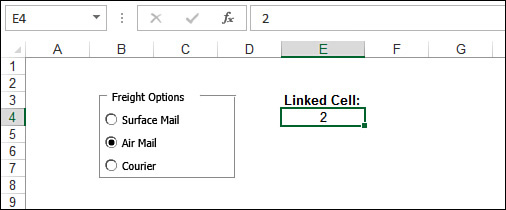
Figure 4.16 For option buttons, the value stored in the linked cell is based on the order in which the buttons were added to the group box.
![]() To learn how to look up values in a worksheet, see Chapter 9, “Working with Lookup Functions,” p. 191.
To learn how to look up values in a worksheet, see Chapter 9, “Working with Lookup Functions,” p. 191.
Check Boxes
Check boxes enable you to include options that the user can toggle on or off. As with option buttons, Excel draws each check box in the unchecked state. If you prefer that a particular check box start in the checked state, use the Format Control dialog box to select the control’s Checked option, as described in the previous section.
On the worksheet, a selected check box stores the value TRUE in its linked cell; if the check box is cleared, it stores the value FALSE (see Figure 4.17). This is handy because it enables you to add a bit of logic to your formulas. That is, you can test whether a check box is selected and adjust a formula accordingly. Figure 4.17 shows a couple examples:
![]() Use End-Of-Period Payments—This check box could be used to specify whether a formula that determines the monthly payments on a loan assumes that those payments are made at the end of each period (
Use End-Of-Period Payments—This check box could be used to specify whether a formula that determines the monthly payments on a loan assumes that those payments are made at the end of each period (TRUE) or at the beginning of each period (FALSE).
![]() Include Extra Monthly Payments—This check box could be used to determine whether a model that builds a loan amortization schedule formula includes an extra principal repayment each month.
Include Extra Monthly Payments—This check box could be used to determine whether a model that builds a loan amortization schedule formula includes an extra principal repayment each month.

Figure 4.17 For check boxes, the value stored in the linked cell is TRUE when the check box is selected and FALSE when it is not selected.
In both cases, and in most formulas that take into account check box results, you would use the IF() worksheet function to read the current value of the linked cell and branch accordingly.
![]() To learn how to use the
To learn how to use the IF() worksheet function, see “Using the IF() Function,” p. 164.
![]() To learn how to build a loan amortization schedule, see “Building a Loan Amortization Schedule,” p. 440.
To learn how to build a loan amortization schedule, see “Building a Loan Amortization Schedule,” p. 440.
List Boxes and Combo Boxes
A list box control creates a list box from which the user can select an item. The items in the list are defined by the values in a specified worksheet range, and the value returned to the linked cell is the number of the item chosen. A combo box is similar to a list box; however, the control shows only one item at a time until it’s dropped down.
List boxes and combo boxes are different from other controls because you also have to specify a range that contains the items to appear in the list. The following steps show you how it’s done:
1. Enter the list items in a range. (The items must be listed in a single row or a single column.)
2. Add the list box control to the sheet (if you haven’t done so already) and then select it.
3. Right-click the control and then click Format Control (or press Ctrl+1) to display the Format Control dialog box.
4. Select the Control tab and then use the Input Range box to enter a reference to the range of items. You can either type in the reference or select it directly on the worksheet.
5. Click OK to return to the worksheet.
Figure 4.18 shows a worksheet with a list box and a drop-down list.
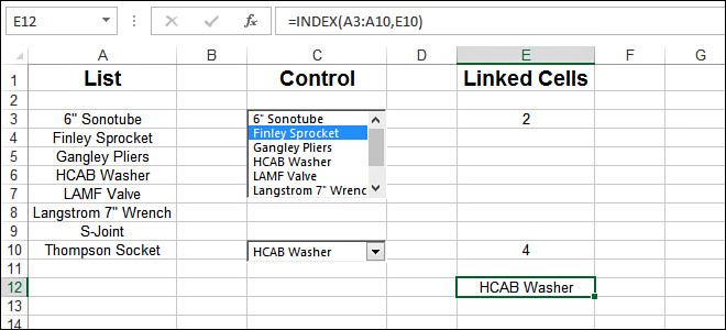
Figure 4.18 For list boxes and combo boxes, the value stored in the linked cell is the number of the selected list item. To get the item text, use the INDEX() function.
The list used by both controls in this example is in the range A3:A10. Notice that the linked cells display the number of the list selection, not the selection itself. To get the selected list item, you can use the INDEX() function with the following syntax:
INDEX(list_range, list_selection)
For example, to find the item that’s currently selected in the combo box in Figure 4.18, you use the following formula (as shown in cell E12):
=INDEX(A3:A10,E10)
![]() To learn more about the
To learn more about the INDEX() function, see Chapter 9, “Working with Lookup Functions,” p. 191.
Scroll Bars and Spin Boxes
The Scroll Bar tool creates a control that resembles a window scroll bar. You use this type of scroll bar to select a number from a range of values. Clicking the arrows or dragging the scroll box changes the value of the control. This value is what gets returned to the linked cell. Note that you can create either a horizontal scroll bar or a vertical scroll bar.
In the Format Control dialog box for a scroll bar, the Control tab includes the following options:
![]() Current Value—The initial value of the scroll bar
Current Value—The initial value of the scroll bar
![]() Minimum Value—The value of the scroll bar when the scroll box is at its leftmost position (for a horizontal scroll bar) or its topmost position (for a vertical scroll bar)
Minimum Value—The value of the scroll bar when the scroll box is at its leftmost position (for a horizontal scroll bar) or its topmost position (for a vertical scroll bar)
![]() Maximum Value—The value of the scroll bar when the scroll box is at its rightmost position (for a horizontal scroll bar) or its bottommost position (for a vertical scroll bar)
Maximum Value—The value of the scroll bar when the scroll box is at its rightmost position (for a horizontal scroll bar) or its bottommost position (for a vertical scroll bar)
![]() Incremental Change—The amount that the scroll bar’s value changes when the user clicks on a scroll arrow
Incremental Change—The amount that the scroll bar’s value changes when the user clicks on a scroll arrow
![]() Page Change—The amount that the scroll bar’s value changes when the user clicks between the scroll box and a scroll arrow
Page Change—The amount that the scroll bar’s value changes when the user clicks between the scroll box and a scroll arrow
The Spin Box tool creates a control that is similar to a scroll bar; that is, you can use a spin box to select a number between a maximum value and a minimum value by clicking the arrows. The number is returned to the linked cell. Spin box options are identical to those of scroll bars, except that you can’t set a Page Change value.
Figure 4.19 shows an example of a scroll bar and an example of a spin box. Note that the numbers above the scroll bar giving the minimum and maximum values are extra labels I added by hand. Doing this is usually a good idea because it gives the user the numeric limits of the control.
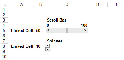
Figure 4.19 For scroll bars and spin boxes, the value stored in the linked cell is the current numeric value of the control.
From Here
![]() To get the details on link formulas, see “Working with Links in Formulas,” p. 70.
To get the details on link formulas, see “Working with Links in Formulas,” p. 70.
![]() To learn about custom numeric formats and to see some examples of using them to display input error messages, see “Formatting Numbers, Dates, and Times,” p. 74.
To learn about custom numeric formats and to see some examples of using them to display input error messages, see “Formatting Numbers, Dates, and Times,” p. 74.
![]() Circular references are usually a bad thing to have in a spreadsheet model. To learn how to combat the bad kind, see “Fixing Circular References,” p. 118.
Circular references are usually a bad thing to have in a spreadsheet model. To learn how to combat the bad kind, see “Fixing Circular References,” p. 118.
![]() To learn how to get Excel to “circle” cells that contain data-validation errors, see “Auditing a Worksheet,” p. 123.
To learn how to get Excel to “circle” cells that contain data-validation errors, see “Auditing a Worksheet,” p. 123.
![]() To learn how to use the
To learn how to use the IF() worksheet function, see “Using the IF() Function,” p. 164.
![]() To learn how to look up values in a worksheet, see Chapter 9, “Working with Lookup Functions,” p. 191.
To learn how to look up values in a worksheet, see Chapter 9, “Working with Lookup Functions,” p. 191.
![]() To learn more about the
To learn more about the INDEX() function, see “The MATCH() and INDEX() Functions,” p. 202.
![]() To learn how the
To learn how the PMT() function works, see “Calculating a Loan Payment,” p. 435.
![]() To learn how to build a loan amortization schedule, see “Building a Loan Amortization Schedule,” p. 440.
To learn how to build a loan amortization schedule, see “Building a Loan Amortization Schedule,” p. 440.