
CHAPTER 13
Partitioning
Partitioning, first introduced in Oracle 8.0, is the process of physically breaking a table or index into many smaller, more manageable pieces. As far as the application accessing the database is concerned, there is logically only one table or one index, but physically that table or index may comprise many dozens of physical partitions. Each partition is an independent object that may be manipulated either by itself or as part of the larger object.
Note Partitioning is an extra cost option to the Enterprise Edition of the Oracle database. It is not available in the Standard Edition.
In this chapter, we will investigate why you might consider using partitioning. The reasons range from increased availability of data to reduced administrative (DBA) burdens and, in certain situations, increased performance. Once you have a good understanding of the reasons for using partitioning, we'll look at how you may partition tables and their corresponding indexes. The goal of this discussion is not to teach you the details of administering partitions, but rather to present a practical guide to implementing your applications with partitions.
We will also discuss the important fact that partitioning of tables and indexes is not a guaranteed "fast = true" setting for the database. It has been my experience that many developers and DBAs believe that increased performance is an automatic side effect of partitioning an object. Partitioning is just a tool, and one of three things will happen when you partition an index or table: the application using these partitioned tables might run slower, might run faster, or might be not be affected one way or the other. I put forth that if you just apply partitioning without understanding how it works and how your application can make use of it, then the odds are you will negatively impact performance by just turning it on.
Lastly, we'll investigate a very common use of partitions in today's world: supporting a large online audit trail in an OLTP and other operational systems. We'll discuss how to incorporate partitioning and segment space compression to efficiently store online a large audit trail and provide the ability to archive old records out of this audit trail with minimal work.
Partitioning Overview
Partitioning facilitates the management of very large tables and indexes using "divide and conquer" logic. Partitioning introduces the concept of a partition key that is used to segregate data based on a certain range value, a list of specific values, or the value of a hash function. If I were to put the benefits of partitioning in some sort of order, it would be
- Increases availability of data: This attribute is applicable to all system types, be they OLTP or warehouse systems by nature.
- Eases administration of large segments by removing them from the database: Performing administrative operations on a 100GB table, such as a reorganization to remove migrated rows or to reclaim "whitespace" left in the table after a purge of old information, would be much more onerous than performing the same operation ten times on individual 10GB table partitions. Additionally, using partitions, we might be able to conduct a purge routine without leaving whitespace behind at all, removing the need for a reorganization entirely!
- Improves the performance of certain queries: This is mainly beneficial in a large warehouse environment where we can use partitioning to eliminate large ranges of data from consideration, avoiding accessing this data at all. This will not be as applicable in a transactional system, since we are accessing small volumes of data in that system already.
- May reduce contention on high-volume OLTP systems by spreading out modifications across many separate partitions: If you have a segment experiencing high contention, turning it into many segments could have the side effect of reducing that contention proportionally.
Let's take a look at each of these potential benefits of using partitioning.
Increased Availability
Increased availability derives from the independence of each partition. The availability (or lack thereof) of a single partition in an object does not mean the object itself is unavailable. The optimizer is aware of the partitioning scheme that is in place and will remove unreferenced partitions from the query plan accordingly. If a single partition is unavailable in a large object, and your query can eliminate this partition from consideration, then Oracle will successfully process the query.
To demonstrate this increased availability, we'll set up a hash partitioned table with two partitions, each in a separate tablespace. We'll create an EMP table that specifies a partition key on the EMPNO column; EMPNO will be our partition key. In this case, this structure means that for each row inserted into this table, the value of the EMPNO column is hashed to determine the partition (and hence the tablespace) into which the row will be placed:
ops$tkyte@ORA10G> CREATE TABLE emp

  2  ( empno  int,

  3    ename  varchar2(20)

  4  )

  5  PARTITION BY HASH (empno)

  6  ( partition part_1 tablespace p1,

  7    partition part_2 tablespace p2

  8  )

  9  /

Table created.
Next, we insert some data into the EMP table and then, using the partition-extended table name, inspect the contents of each partition:
ops$tkyte@ORA10G> insert into emp select empno, ename from scott.emp

  2 /

14 rows created.


ops$tkyte@ORA10G> select * from emp partition(part_1);


     EMPNO ENAME

---------- --------------------

      7369 SMITH

      7499 ALLEN

      7654 MARTIN

      7698 BLAKE

      7782 CLARK

      7839 KING

      7876 ADAMS

      7934 MILLER

8 rows selected.


ops$tkyte@ORA10G> select * from emp partition(part_2);


   EMPNO ENAME

---------- --------------------

    7521 WARD

    7566 JONES

    7788 SCOTT

    7844 TURNER

    7900 JAMES

    7902 FORD

6 rows selected.
You should note that the data is somewhat randomly assigned. That is by design here. Using hash partitioning, we are asking Oracle to randomly—but hopefully evenly—distribute our data across many partitions. We cannot control the partition into which data goes; Oracle decides that based on the hash key values that it generates. Later, when we look at range and list partitioning, we'll see how we can control what partitions receive which data.
Now, we take one of the tablespaces offline (simulating, for example, a disk failure), thus making the data unavailable in that partition:
ops$tkyte@ORA10G> alter tablespace p1 offline;

Tablespace altered.
Next, we run a query that hits every partition, and we see that this query fails:
ops$tkyte@ORA10G> select * from emp;

select * from emp

              *

ERROR at line 1:

ORA-00376: file 12 cannot be read at this time

ORA-01110: data file 12:

'/home/ora10g/oradata/ora10g/ORA10G/datafile/p1.dbf'
However, a query that does not access the offline tablespace will function as normal; Oracle will eliminate the offline partition from consideration. I use a bind variable in this particular example just to demonstrate that even though Oracle does not know at query optimization time which partition will be accessed, it is nonetheless able to perform this elimination at runtime:
ops$tkyte@ORA10G> variable n number

ops$tkyte@ORA10G> exec :n := 7844;

PL/SQL procedure successfully completed.


ops$tkyte@ORA10G> select * from emp where empno = :n;


     EMPNO ENAME

---------- --------------------

      7844 TURNER
In summary, when the optimizer can eliminate partitions from the plan, it will. This fact increases availability for those applications that use the partition key in their queries.
Partitions also increase availability by reducing downtime. If you have a 100GB table, for example, and it is partitioned into 50 2GB partitions, then you can recover from errors that much faster. If one of the 2GB partitions is damaged, the time to recover is now the time it takes to restore and recover a 2GB partition, not a 100GB table. So availability is increased in two ways:
- Partition elimination by the optimizer means that many users may never even notice that some of the data was unavailable.
- Downtime is reduced in the event of an error because of the significantly reduced amount of work that is required to recover.
Reduced Administrative Burden
The administrative burden relief is derived from the fact that performing operations on small objects is inherently easier, faster, and less resource intensive than performing the same operation on a large object.
For example, say you have a 10GB index in your database. If you need to rebuild this index and it is not partitioned, then you will have to rebuild the entire 10GB index as a single unit of work. While it is true that you could rebuild the index online, it requires a huge number of resources to completely rebuild an entire 10GB index. You'll need at least 10GB of free storage elsewhere to hold a copy of both indexes, you'll need a temporary transaction log table to record the changes made against the base table during the time you spend rebuilding the index, and so on. On the other hand, if the index itself had been partitioned into ten 1GB partitions, then you could rebuild each index partition individually, one by one. Now you need 10 percent of the free space you needed previously. Likewise, the individual index rebuilds will each be much faster (ten times faster, perhaps), so far fewer transactional changes occurring during an online index rebuild need to be merged into the new index, and so on.
Also, consider what happens in the event of a system or software failure just before completing the rebuilding of a 10GB index. The entire effort is lost. By breaking the problem down and partitioning the index into 1GB partitions, at most you would lose 10 percent of the total work required to rebuild the index.
Alternatively, it may be that you need to rebuild only 10 percent of the total aggregate index—for example, only the "newest" data (the active data) is subject to this reorganization, and all of the "older" data (which is relatively static) remains unaffected.
Finally, consider the situation whereby you discover 50 percent of the rows in your table are "migrated" rows (see Chapter 10 for details on chained/migrated rows), and you would like to fix this. Having a partitioned table will facilitate the operation. To "fix" migrated rows, you must typically rebuild the object—in this case, a table. If you have one 100GB table, you will need to perform this operation in one very large "chunk," serially, using ALTER TABLE MOVE. On the other hand, if you have 25 partitions, each 4GB in size, then you can rebuild each partition one by one. Alternatively, if you are doing this during off-hours and have ample resources, you can even do the ALTER TABLE MOVE statements in parallel, in separate sessions, potentially reducing the amount of time the whole operation will take. Virtually everything you can do to a nonpartitioned object, you can do to an individual partition of a partitioned object. You might even discover that your migrated rows are concentrated in a very small subset of your partitions, hence you could rebuild one or two partitions instead of the entire table.
Here is a quick example demonstrating the rebuild of a table with many migrated rows. Both BIG_TABLE1 and BIG_TABLE2 were created from a 10,000,000-row instance of BIG_TABLE (see the "Setup" section for the BIG_TABLE creation script). BIG_TABLE1 is a regular, nonpartitioned table, whereas BIG_TABLE2 is a hash partitioned table in eight partitions (we'll cover hash partitioning in a subsequent section; suffice it to say, it distributed the data rather evenly into eight partitions):
ops$tkyte@ORA10GR1> create table big_table1

  2  ( ID, OWNER, OBJECT_NAME, SUBOBJECT_NAME,

  3    OBJECT_ID, DATA_OBJECT_ID,

  4    OBJECT_TYPE, CREATED, LAST_DDL_TIME,

  5    TIMESTAMP, STATUS, TEMPORARY,

  6    GENERATED, SECONDARY )

  7  tablespace big1

  8  as

  9  select ID, OWNER, OBJECT_NAME, SUBOBJECT_NAME,

 10         OBJECT_ID, DATA_OBJECT_ID,

 11         OBJECT_TYPE, CREATED, LAST_DDL_TIME,

 12         TIMESTAMP, STATUS, TEMPORARY,

 13         GENERATED, SECONDARY

 14    from big_table.big_table;

Table created.

ops$tkyte@ORA10GR1> create table big_table2

  2  ( ID, OWNER, OBJECT_NAME, SUBOBJECT_NAME,

  3    OBJECT_ID, DATA_OBJECT_ID,

  4    OBJECT_TYPE, CREATED, LAST_DDL_TIME,

  5    TIMESTAMP, STATUS, TEMPORARY,

  6    GENERATED, SECONDARY )

  7  partition by hash(id)

  8  (partition part_1 tablespace big2,

  9   partition part_2 tablespace big2,

 10   partition part_3 tablespace big2,

 11   partition part_4 tablespace big2,

 12   partition part_5 tablespace big2,

 13   partition part_6 tablespace big2,

 14   partition part_7 tablespace big2,

 15   partition part_8 tablespace big2

 16  )

 17  as

 18  select ID, OWNER, OBJECT_NAME, SUBOBJECT_NAME,

 19         OBJECT_ID, DATA_OBJECT_ID,

 20         OBJECT_TYPE, CREATED, LAST_DDL_TIME,

 21         TIMESTAMP, STATUS, TEMPORARY,

 22         GENERATED, SECONDARY

 23    from big_table.big_table;

Table created.
Now, each of those tables is in its own tablespace, so we can easily query the data dictionary to see the allocated and free space in each tablespace:
ops$tkyte@ORA10GR1> select b.tablespace_name,

  2         mbytes_alloc,

  3         mbytes_free

  4    from ( select round(sum(bytes)/1024/1024) mbytes_free,

  5                  tablespace_name

  6             from dba_free_space

  7            group by tablespace_name ) a,

  8         ( select round(sum(bytes)/1024/1024) mbytes_alloc,

  9                  tablespace_name

 10             from dba_data_files

 11            group by tablespace_name ) b

 12   where a.tablespace_name (+) = b.tablespace_name

 13     and b.tablespace_name in ('BIG1','BIG2')

 14 /


TABLESPACE MBYTES_ALLOC MBYTES_FREE

---------- ------------ -----------

BIG1               1496         344

BIG2               1496         344
BIG1 and BIG2 are both about 1.5GB in size and each have 344MB free. We'll try to rebuild the first table, BIG_TABLE1:
ops$tkyte@ORA10GR1> alter table big_table1 move;

alter table big_table1 move

            *

ERROR at line 1:

ORA-01652: unable to extend temp segment by 1024 in tablespace BIG1
That fails—we needed sufficient free space in tablespace BIG1 to hold an entire copy of BIG_TABLE1 at the same time as the old copy was there—in short, we would need about two times the storage for a short period (maybe more, maybe less—it depends on the resulting size of the rebuilt table). We now attempt the same operation on BIG_TABLE2:
ops$tkyte@ORA10GR1> alter table big_table2 move;

alter table big_table2 move

            *

ERROR at line 1:

ORA-14511: cannot perform operation on a partitioned object
That is Oracle telling us we cannot do the MOVE operation on the "table"; we must perform the operation on each partition of the table instead. We can move (hence rebuild and reorganize) each partition one by one:
ops$tkyte@ORA10GR1> alter table big_table2 move partition part_1;

Table altered.

ops$tkyte@ORA10GR1> alter table big_table2 move partition part_2;

Table altered.

ops$tkyte@ORA10GR1> alter table big_table2 move partition part_3;

Table altered.

ops$tkyte@ORA10GR1> alter table big_table2 move partition part_4;

Table altered.

ops$tkyte@ORA10GR1> alter table big_table2 move partition part_5;

Table altered.

ops$tkyte@ORA10GR1> alter table big_table2 move partition part_6;

Table altered.

ops$tkyte@ORA10GR1> alter table big_table2 move partition part_7;

Table altered.

ops$tkyte@ORA10GR1> alter table big_table2 move partition part_8;

Table altered.
Each individual move only needed sufficient free space to hold a copy of one-eighth of the data! Therefore, these commands succeeded given the same amount of free space as we had before. We needed significantly less temporary resources and, further, if the system failed (e.g., due to a power outage) after we moved PART_4 but before PART_5 finished "moving," we would not have lost all of the work performed as we would have with a single MOVE statement. The first four partitions would still be "moved" when the system recovered, and we may resume processing at partition PART_5.
Some may look at that and say, "Wow, eight statements—that is a lot of typing," and it's true that this sort of thing would be unreasonable if you had hundreds of partitions (or more). Fortunately, it is very easy to script a solution, and the previous would become simply
ops$tkyte@ORA10GR1> begin

  2      for x in ( select partition_name

  3                   from user_tab_partitions

  4                  where table_name = 'BIG_TABLE2' )

  5      loop

  6          execute immediate

  7          'alter table big_table2 move partition ' ||

  8           x.partition_name;

  9      end loop;

 10  end;

 11  /

PL/SQL procedure successfully completed.
All of the information you need is there in the Oracle data dictionary, and most sites that have implemented partitioning also have a series of stored procedures they use to make managing large numbers of partitions easy. Additionally, many GUI tools such as Enterprise Manager have the built-in capability to perform these operations as well, without your needing to type in the individual commands.
Another factor to consider with regard to partitions and administration is the use of "sliding windows" of data in data warehousing and archiving. In many cases, you need to keep data online that spans the last N units of time. For example, say you need to keep the last 12 months or the last 5 years online. Without partitions, this is generally a massive INSERT followed by a massive DELETE. Lots of DML, and lots of redo and undo generated. Now with partitions, you can simply do the following:
- Load a separate table with the new months' (or years', or whatever) data.
- Index the table fully. (These steps could even be done in another instance and transported to this database.)
- Attach this newly loaded and indexed table onto the end of the partitioned table using a fast DDL command:
ALTER TABLE EXCHANGE PARTITION. - Detach the oldest partition off the other end of the partitioned table.
So, you can now very easily support extremely large objects containing time-sensitive information. The old data can easily be removed from the partitioned table and simply dropped if you do not need it, or it can be archived off elsewhere. New data can be loaded into a separate table, so as to not affect the partitioned table until the loading, indexing, and so on is complete. We will take a look at a complete example of a sliding window later in this chapter.
In short, partitioning can make what would otherwise be daunting, or in some cases unfeasible, operations as easy as they are in a small database.
Enhanced Statement Performance
The last general (potential) benefit of partitioning is in the area of enhanced statement (SELECT, INSERT, UPDATE, DELETE, MERGE) performance. We'll take a look at two classes of statements—those that modify information and those that just read information—and discuss what benefits we might expect from partitioning in each case.
Parallel DML
Statements that modify data in the database may have the potential to perform parallel DML (PDML). During PDML, Oracle uses many threads or processes to perform your INSERT, UPDATE, or DELETE instead of a single serial process. On a multi-CPU machine with plenty of I/O bandwidth, the potential increase in speed may be large for mass DML operations. In releases of Oracle prior to 9i, PDML required partitioning. If your tables were not partitioned, you could not perform these operations in parallel in the earlier releases. If the tables were partitioned, Oracle would assign a maximum degree of parallelism to the object, based on the number of physical partitions it had. This restriction was, for the most part, relaxed in Oracle9i and later with two notable exceptions. If the table you wish to perform PDML on has a bitmap index in place of a LOB column, then the table must be partitioned in order to have the operation take place in parallel, and the degree of parallelism will be restricted to the number of partitions. In general, though, you no longer need to partition to use PDML.
Note We will cover parallel operations in more detail in Chapter 14.
Query Performance
In the area of strictly read query performance (SELECT statements), partitioning comes into play with two types of specialized operations:
- Partition elimination: Some partitions of data are not considered in the processing of the query. We have already seen an example of partition elimination.
- Parallel operations: Examples of this are parallel full table scans and parallel index range scans.
However, the benefit you can derive from these depends very much on the type of system you are using.
OLTP Systems
You should not look toward partitions as a way to massively improve query performance in an OLTP system. In fact, in a traditional OLTP system, you must apply partitioning with care so as to not negatively affect runtime performance. In a traditional OLTP system, most queries are expected to return virtually instantaneously, and most of the retrievals from the database are expected to be via very small index range scans. Therefore, the main performance benefits of partitioning listed previously would not come into play. Partition elimination is useful where you have full scans of large objects, because it allows you to avoid full scanning large pieces of an object. However, in an OLTP environment, you are not full scanning large objects (if you are, you have a serious design flaw). Even if you partition your indexes, any increase in performance achieved by scanning a smaller index will be miniscule—if you actually achieve an increase in speed at all. If some of your queries use an index and they cannot eliminate all but one partition from consideration, you may find your queries actually run slower after partitioning since you now have 5, 10, or 20 small indexes to probe, instead of one larger index. We will investigate this in much more detail shortly when we look at the types of partitioned indexes available to us.
Having said all this, there are opportunities to gain efficiency in an OLTP system with partitions. For example, they may be used to increase concurrency by decreasing contention. They can be used to spread out the modifications of a single table over many physical partitions. Instead of having a single table segment with a single index segment, you might have 20 table partitions and 20 index partitions. It could be like having 20 tables instead of 1, hence contention would be decreased for this shared resource during modifications.
As for parallel operations, as we'll investigate in more detail in the next chapter, you do not want to do a parallel query in an OLTP system. You would reserve your use of parallel operations for the DBA to perform rebuilds, create indexes, gather statistics, and so on. The fact is that in an OLTP system, your queries should already be characterized by very fast index accesses, and partitioning will not speed that up very much, if at all. This does not mean that you should avoid partitioning for OLTP; it means that you shouldn't expect partitioning to offer massive improvements in performance. Most OLTP applications are not able to take advantage of the times where partitioning is able to enhance query performance, but you can still benefit from the other two possible partitioning benefits; administrative ease and higher availability.
Data Warehouse Systems
In a data warehouse/decision-support system, partitioning is not only a great administrative tool, but also something that will speed up processing. For example, you may have a large table on which you need to perform an ad hoc query. You always do the ad hoc query by sales quarter, as each sales quarter contains hundreds of thousands of records and you have millions of online records. So, you want to query a relatively small slice of the entire data set, but it is not really feasible to index it based on the sales quarter. This index would point to hundreds of thousands of records, and doing the index range scan in this way would be terrible (refer to Chapter 11 for more details on this). A full table scan is called for to process many of your queries, but you end up having to scan millions of records, most of which won't apply to our query. Using an intelligent partitioning scheme, you can segregate the data by quarter such that when you query the data for any given quarter, you will full scan only that quarter's data. This is the best of all possible solutions.
In addition, in a data warehouse/decision-support system environment, parallel query is used frequently. Here, operations such as parallel index range scans or parallel fast full index scans are not only meaningful, but also beneficial to us. We want to maximize our use of all available resources, and parallel query is a way to do it. So, in this environment, partitioning stands a very good chance of speeding up processing.
Table Partitioning Schemes
There are currently four methods by which you can partition tables in Oracle:
- Range partitioning: You may specify ranges of data that should be stored together. For example, everything that has a timestamp within the month of
Jan-2005will be stored in partition 1, everything with a timestamp withinFeb-2005will be stored in partition 2, and so on. This is probably the most commonly used partitioning mechanism in Oracle. - Hash partitioning: You saw this in the first example in this chapter. A column (or columns) has a hash function applied to it, and the row will be placed into a partition according to the value of this hash.
- List partitioning: You specify a discrete set of values, which determines the data that should be stored together. For example, you could specify that rows with a
STATUScolumn value in( 'A', 'M', 'Z' )go into partition 1, those with aSTATUSvalue in( 'D', 'P', 'Q' )go into partition 2, and so on. - Composite partitioning: This is a combination of range and hash or range and list. It allows you to first apply range partitioning to some data, and then within that range have the final partition be chosen by hash or list.
In the following sections, we'll look at the benefits of each type of partitioning and at the differences between them. We'll also look at when to apply which schemes to different application types. This section is not intended to present a comprehensive demonstration of the syntax of partitioning and all of the available options. Rather, the examples are simple and illustrative, and designed to give you an overview of how partitioning works and how the different types of partitioning are designed to function.
Note For full details on partitioning syntax, I refer you to either the Oracle SQL Reference Guide or to the Oracle Administrator's Guide. Additionally, the Oracle Data Warehousing Guide is an excellent source of information on the partitioning options and is a must-read for anyone planning to implement partitioning.
Range Partitioning
The first type we will look at is a range partitioned table. The following CREATE TABLE statement creates a range partitioned table using the column RANGE_KEY_COLUMN. All data with a RANGE_KEY_COLUMN strictly less than 01-JAN-2005 will be placed into the partition PART_1, and all data with a value strictly less than 01-JAN-2006 will go into partition PART_2. Any data not satisfying either of those conditions (e.g., a row with a RANGE_KEY_COLUMN value of 01-JAN-2007) will fail upon insertion, as it cannot be mapped to a partition:
ops$tkyte@ORA10GR1> CREATE TABLE range_example

  2  ( range_key_column date,

  3    data             varchar2(20)

  4  )

  5  PARTITION BY RANGE (range_key_column)

  6  ( PARTITION part_1 VALUES LESS THAN

  7         (to_date('01/01/2005','dd/mm/yyyy')),

  8    PARTITION part_2 VALUES LESS THAN

  9         (to_date('01/01/2006','dd/mm/yyyy'))

 10 )

 11 /

Table created.
Note We are using the date format DD/MM/YYYY in the CREATE TABLE to make this "international." If we used a format of DD-MON-YYYY, then the CREATE TABLE would fail with ORA-01843: not a valid month if the abbreviation of January was not Jan on your system. The NLS_LANGUAGE setting would affect this. I have used the three-character month abbreviation in the text and inserts, however, to avoid any ambiguity as to which component is the day and which is the month.
Figure 13-1 shows that Oracle will inspect the value of the RANGE_KEY_COLUMN and, based on that value, insert it into one of the two partitions.
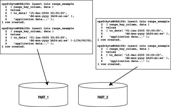
Figure 13-1. Range partition insert example
The rows inserted were specifically chosen with the goal of demonstrating that the partition range is strictly less than and not less than or equal to. We first insert the value 15-DEC-2004, which will definitely go into partition PART_1. We also insert a row with a date/time that is one second before 01-JAN-2005—that row will also will go into partition PART_1 since that is less than 01-JAN-2005. However, the next insert of midnight on 01-JAN-2005 goes into partition PART_2 because that date/time is not strictly less than the partition range boundary. The last row obviously belongs in partition PART_2 since it is less than the partition range boundary for PART_2.
We can confirm that this is the case by performing SELECT statements from the individual partitions:
ops$tkyte@ORA10G> select to_char(range_key_column,'dd-mon-yyyy hh24:mi:ss')

  2    from range_example partition (part_1);


TO_CHAR(RANGE_KEY_CO

--------------------

15-dec-2004 00:00:00

31-dec-2004 23:59:59


ops$tkyte@ORA10G> select to_char(range_key_column,'dd-mon-yyyy hh24:mi:ss')

  2    from range_example partition (part_2);


TO_CHAR(RANGE_KEY_CO

--------------------

01-jan-2005 00:00:00

15-dec-2005 00:00:00
You might be wondering what would happen if you inserted a date that fell outside of the upper bound. The answer is that Oracle will raise an error:
ops$tkyte@ORA10GR1> insert into range_example

  2  ( range_key_column, data )

  3  values

  4  ( to_date( '15/12/2007 00:00:00',

  5             'dd/mm/yyyy hh24:mi:ss' ),

  6    'application data...' );

insert into range_example

            *

ERROR at line 1:

ORA-14400: inserted partition key does not map to any partition
Suppose you want to segregate 2005 and 2006 dates into their separate partitions as we have, but you want all other dates to go into a third partition. With range partitioning, you can do this using the MAXVALUE clause, which looks like this:
ops$tkyte@ORA10GR1> CREATE TABLE range_example

  2  ( range_key_column date,

  3    data             varchar2(20)

  4  )

  5  PARTITION BY RANGE (range_key_column)

  6  ( PARTITION part_1 VALUES LESS THAN

  7         (to_date('01/01/2005','dd/mm/yyyy')),

  8    PARTITION part_2 VALUES LESS THAN

  9         (to_date('01/01/2006','dd/mm/yyyy'))

 10    PARTITION part_3 VALUES LESS THAN

 11         (MAXVALUE)

 12  )

 13  /


Table created.
Now when you insert a row into that table, it will go into one of the three partitions—no row will be rejected, since partition PART_3 can take any value of RANGE_KEY_COLUMN that doesn't go into PART_1 or PART_2 (even null values of the RANGE_KEY_COLUMN will be inserted into this new partition).
Hash Partitioning
When hash partitioning a table, Oracle will apply a hash function to the partition key to determine in which of the N partitions the data should be placed. Oracle recommends that N be a number that is a power of 2 (2, 4, 8, 16, and so on) to achieve the best overall distribution, and we'll see shortly that this is absolutely good advice.
How Hash Partitioning Works
Hash partitioning is designed to achieve a good spread of data across many different devices (disks), or just to segregate data out into more manageable chunks. The hash key chosen for a table should be a column or set of columns that are unique, or at least have as many distinct values as possible to provide for a good spread of the rows across partitions. If you choose a column that has only four values, and you use two partitions, then all the rows could quite easily end up hashing to the same partition, obviating the goal of partitioning in the first place!
We will create a hash table with two partitions in this case. We will use a column named HASH_KEY_COLUMN as our partition key. Oracle will take the value in this column and determine the partition this row will be stored in by hashing that value:
ops$tkyte@ORA10G> CREATE TABLE hash_example

  2  ( hash_key_column  date,

  3    data             varchar2(20)

  4  )

  5  PARTITION BY HASH (hash_key_column)

  6  ( partition part_1 tablespace p1,

  7   partition part_2 tablespace p2

  8  )

  9  /

Table created.
Figure 13-2 shows that Oracle will inspect the value in the HASH_KEY_COLUMN, hash it, and determine which of the two partitions a given row will appear in:
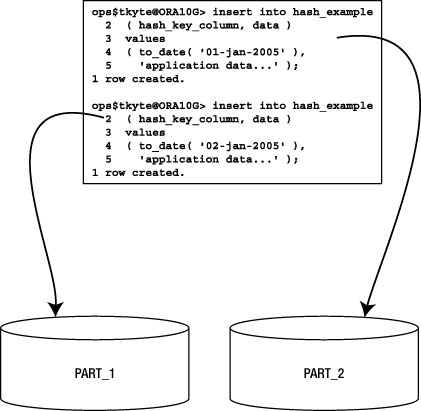
Figure 13-2. Hash partition insert example
As noted earlier, hash partitioning gives you no control over which partition a row ends up in. Oracle applies the hash function and the outcome of that hash determines where the row goes. If you want a specific row to go into partition PART_1 for whatever reason, you should not—in fact, you cannot—use hash partitioning. The row will go into whatever partition the hash function says to put it in. If you change the number of hash partitions, the data will be redistributed over all of the partitions (adding or removing a partition to a hash partitioned table will cause all of the data to be rewritten, as every row may now belong in a different partition).
Hash partitioning is most useful when you have a large table, such as the one shown in the "Reduced Administrative Burden" section, and you would like to "divide and conquer" it. Rather than manage one large table, you would like to have 8 or 16 smaller "tables" to manage. Hash partitioning is also useful to increase availability to some degree, as demonstrated in the "Increased Availability" section; the temporary loss of a single hash partition permits access to all of the remaining partitions. Some users may be affected, but there is a good chance that many will not be. Additionally, the unit of recovery is much smaller now. You do not have a single large table to restore and recover; you have a fraction of that table to recover. Lastly, hash partitioning is useful in high update contention environments, as mentioned in the "Enhanced Statement Performance" section when we talked about OLTP systems. Instead of having a single "hot" segment, we can hash partition a segment into 16 pieces, each of which is now receiving modifications.
Hash Partition Using Powers of Two
I mentioned earlier that the number of partitions should be a power of two. This is easily observed to be true. To demonstrate, we'll set up a stored procedure to automate the creation of a hash partitioned table with N partitions (N will be a parameter). This procedure will construct a dynamic query to retrieve the counts of rows by partition and then display the counts and a simple histogram of the counts by partition. Lastly, it will open this query and let us see the results. This procedure starts with the hash table creation. We will use a table named T:
ops$tkyte@ORA10G> create or replace

  2  procedure hash_proc

  3            ( p_nhash in number,

  4              p_cursor out sys_refcursor )

  5  authid current_user

  6  as

  7      l_text     long;

  8      l_template long :=

  9             'select $POS$ oc, ''p$POS$'' pname, count(*) cnt ' ||

 10               'from t partition ( $PNAME$ ) union all ';

 11  begin

 12      begin

 13          execute immediate 'drop table t';

 14      exception when others

 15          then null;

 16      end;

 17

 18      execute immediate '

 19      CREATE TABLE t ( id )

 20      partition by hash(id)

 21      partitions ' || p_nhash || '

 22      as

 23      select rownum

 24        from all_objects';
Next, we will dynamically construct a query to retrieve the count of rows by partition. It does this using the "template" query defined earlier. For each partition, we'll gather the count using the partition-extended table name and union all of the counts together:
 25

 26   for x in ( select partition_name pname,

 27                     PARTITION_POSITION pos

 28                from user_tab_partitions

 29               where table_name = 'T'

 30               order by partition_position )

 31   loop

 32       l_text := l_text ||

 33                 replace(

 34                 replace(l_template,

 35                  '$POS$', x.pos),

 36                  '$PNAME$', x.pname );

 37    end loop;
Now, we'll take that query and select out the partition position (PNAME) and the count of rows in that partition (CNT). Using RPAD, we'll construct a rather rudimentary but effective histogram:
 38

 39      open p_cursor for

 40         'select pname, cnt,

 41            substr( rpad(''*'',30*round( cnt/max(cnt)over(),2),''*''),1,30) hg

 42            from (' || substr( l_text, 1, length(l_text)-11 ) || ')

 43           order by oc';

 44

 45  end;

 46  /

Procedure created.
If we run this with an input of 4, for four hash partitions, we would expect to see output similar to the following:
ops$tkyte@ORA10G> variable x refcursor

ops$tkyte@ORA10G> set autoprint on

ops$tkyte@ORA10G> exec hash_proc( 4, :x );

PL/SQL procedure successfully completed.


PN        CNT HG

-- ---------- ------------------------------

p1      12141 *****************************

p2      12178 *****************************

p3      12417 ******************************

p4      12105 *****************************
The simple histogram depicted shows a nice, even distribution of data over each of the four partitions. Each has close to the same number of rows in it. However, if we simply go from four to five hash partitions, we'll see the following:
ops$tkyte@ORA10G> exec hash_proc( 5, :x );

PL/SQL procedure successfully completed.


PN        CNT HG

-- ---------- ------------------------------

p1       6102 **************

p2      12180 *****************************

p3      12419 ******************************

p4      12106 *****************************

p5       6040 **************
This histogram points out that the first and last partitions have just half as many rows as the interior partitions. The data is not very evenly distributed at all. We'll see the trend continue for six and seven hash partitions:
ops$tkyte@ORA10G> exec hash_proc( 6, :x );

PL/SQL procedure successfully completed.


PN        CNT HG

-- ---------- ------------------------------

p1       6104 **************

p2       6175 ***************

p3      12420 ******************************

p4      12106 *****************************

p5       6040 **************

p6       6009 **************

6 rows selected.


ops$tkyte@ORA10G> exec hash_proc( 7, :x );

PL/SQL procedure successfully completed.


PN        CNT HG

-- ---------- ------------------------------

p1       6105 ***************

p2       6176 ***************

p3       6161 ***************

p4      12106 ******************************

p5       6041 ***************

p6       6010 ***************

p7       6263 ***************

7 rows selected.
As soon as we get back to a number of hash partitions that is a power of two, we achieve the goal of even distribution once again:
ops$tkyte@ORA10G> exec hash_proc( 8, :x );

PL/SQL procedure successfully completed.


PN        CNT HG

-- ---------- ------------------------------

p1       6106 *****************************

p2       6178 *****************************

p3       6163 *****************************

p4       6019 ****************************

p5       6042 ****************************

p6       6010 ****************************

p7       6264 ******************************

p8       6089 *****************************

8 rows selected.
If you continue this experiment up to 16 partitions, you would see the same effects for the ninth through the fifteenth partitions—a skewing of the data to the interior partitions, away from the edges, and then upon hitting the sixteenth partition you would see a flattening-out again. The same would be true again up to 32 partitions, and then 64, and so on. This example just points out the importance of using a power of two as the number of hash partitions.
List Partitioning
List partitioning was a new feature of Oracle9i Release 1. It provides the ability to specify in which partition a row will reside, based on discrete lists of values. It is often useful to be able to partition by some code, such as a state or region code. For example, you might want to pull together in a single partition all records for people in the states of Maine (ME), New Hampshire (NH), Vermont (VT), and Massachusetts (MA), since those states are located next to or near each other, and your application queries data by geographic region. Similarly, you might want to group together Connecticut (CT), Rhode Island (RI), and New York (NY).
You cannot use a range partition, since the range for the first partition would be ME through VT, and the second range would be CT through RI. Those ranges overlap. You cannot use hash partitioning since you cannot control which partition any given row goes into; the built-in hash function provided by Oracle does that.
With list partitioning, we can accomplish this custom partitioning scheme easily:
ops$tkyte@ORA10G> create table list_example

  2  ( state_cd   varchar2(2),

  3    data       varchar2(20)

  4  )

  5  partition by list(state_cd)

  6  ( partition part_1 values ( 'ME', 'NH', 'VT', 'MA' ),

  7    partition part_2 values  ( 'CT', 'RI', 'NY' )

  8  )

  9  /

Table created.
Figure 13-3 shows that Oracle will inspect the STATE_CD column and, based on its value, place the row into the correct partition.
As we saw for range partitioning, if we try to insert a value that isn't specified in the list partition, Oracle will raise an appropriate error back to the client application. In other words, a list partitioned table without a DEFAULT partition will implicitly impose a constraint much like a check constraint on the table:
ops$tkyte@ORA10G> insert into list_example values ( 'VA', 'data' );

insert into list_example values ( 'VA', 'data' )

            *

ERROR at line 1:

ORA-14400: inserted partition key does not map to any partition
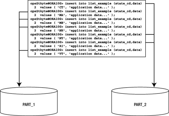
Figure 13-3. List partition insert example
If you want to segregate these seven states into their separate partitions, as we have, but have all remaining state codes (or, in fact, any other row that happens to be inserted that doesn't have one of these seven codes) go into a third partition, then we can use the VALUES ( DEFAULT ) clause. Here, we'll alter the table to add this partition (we could use this in the CREATE TABLE statement as well):
ops$tkyte@ORA10G> alter table list_example

  2  add partition

  3  part_3 values ( DEFAULT );

Table altered.


ops$tkyte@ORA10G> insert into list_example values ( 'VA', 'data' );

1 row created.
All values that are not explicitly in our list of values will go here. A word of caution on the use of DEFAULT: once a list partitioned table has a DEFAULT partition, you cannot add any more partitions to it:
ops$tkyte@ORA10G> alter table list_example

  2  add partition

  3  part_4 values( 'CA', 'NM' );

alter table list_example

            *

ERROR at line 1:

ORA-14323: cannot add partition when DEFAULT partition exists
We would have to remove the DEFAULT partition, then add PART_4, and then put the DEFAULT partition back. The reason behind this is that the DEFAULT partition could have had rows with the list partition key value of CA or NM—they would not belong in the DEFAULT partition after adding PART_4.
Composite Partitioning
Lastly, we'll look at some examples of composite partitioning, which is a mixture of range and hash or range and list.
In composite partitioning, the top-level partitioning scheme is always range partitioning. The secondary level of partitioning is either list or hash (in Oracle9i Release 1 and earlier only hash subpartitioning is supported, not list). It is interesting to note that when you use composite partitioning, there will be no partition segments—there will be only subpartition segments. When using composite partitioning, the partitions themselves do not have segments (much like a partitioned table doesn't have a segment). The data is physically stored in subpartition segments and the partition becomes a logical container, or a container that points to the actual subpartitions.
In our example, we'll look at a range-hash composite. Here we are using a different set of columns for the range partition from those used for the hash partition. This is not mandatory; we could use the same set of columns for both:
ops$tkyte@ORA10G> CREATE TABLE composite_example

  2  ( range_key_column   date,

  3    hash_key_column    int,

  4    data               varchar2(20)

  5  )

  6  PARTITION BY RANGE (range_key_column)

  7  subpartition by hash(hash_key_column) subpartitions 2

  8  (

  9  PARTITION part_1

 10       VALUES LESS THAN(to_date('01/01/2005','dd/mm/yyyy'))

 11       (subpartition part_1_sub_1,

 12        subpartition part_1_sub_2

 13       ),

 14  PARTITION part_2

 15      VALUES LESS THAN(to_date('01/01/2006','dd/mm/yyyy'))

 16      (subpartition part_2_sub_1,

 17       subpartition part_2_sub_2

 18      )

 19  )

 20  /

Table created.
In range-hash composite partitioning, Oracle will first apply the range partitioning rules to figure out which range the data falls into. Then it will apply the hash function to decide into which physical partition the data should finally be placed. This process is described in Figure 13-4.
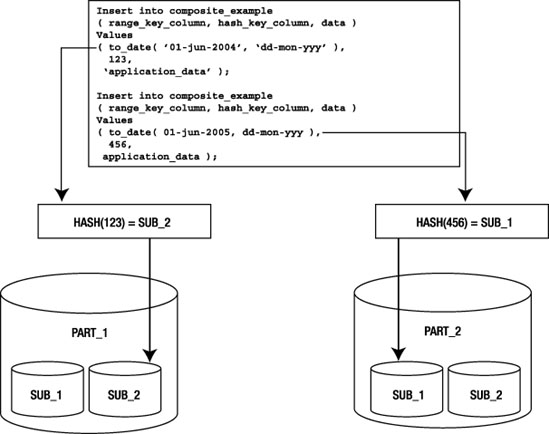
Figure 13-4. Range-hash composite partition example
So, composite partitioning gives you the ability to break up your data by range and, when a given range is considered too large or further partition elimination could be useful, to break it up further by hash or list. It is interesting to note that each range partition need not have the same number of subpartitions; for example, suppose you were range partitioning on a date column in support of data purging (to remove all old data rapidly and easily). In the year 2004, you had equal amounts of data in "odd" code numbers in the CODE_KEY_COLUMN and in "even" code numbers. But in 2005, you knew the number of records associated with the odd code number was more than double, and you wanted to have more subpartitions for the odd code values. You can achieve that rather easily just by defining more subpartitions:
ops$tkyte@ORA10G> CREATE TABLE composite_range_list_example

   2  ( range_key_column   date,

   3    code_key_column    int,

   4    data               varchar2(20)

   5  )

   6  PARTITION BY RANGE (range_key_column)

   7  subpartition by list(code_key_column)

   8  (

   9  PARTITION part_1

 10       VALUES LESS THAN(to_date('01/01/2005','dd/mm/yyyy'))

 11       (subpartition part_1_sub_1 values( 1, 3, 5, 7 ),

 12        subpartition part_1_sub_2 values( 2, 4, 6, 8 )

 13       ),

 14  PARTITION part_2

 15      VALUES LESS THAN(to_date('01/01/2006','dd/mm/yyyy'))

 16      (subpartition part_2_sub_1 values ( 1, 3 ),

 17       subpartition part_2_sub_2 values ( 5, 7 ),

 18       subpartition part_2_sub_3 values ( 2, 4, 6, 8 )

 19      )

 20  )

 21  /

Table created.
Here you end up with five partitions altogether: two subpartitions for partition PART_1 and three for partition PART_2.
Row Movement
You might wonder what would happen if the column used to determine the partition is modified in any of the preceding partitioning schemes. There are two cases to consider:
- The modification would not cause a different partition to be used; the row would still belong in this partition. This is supported in all cases.
- The modification would cause the row to move across partitions. This is supported if row movement is enabled for the table; otherwise, an error will be raised.
We can observe these behaviors easily. In the previous example, we inserted a pair of rows into PART_1 of the RANGE_EXAMPLE table:
ops$tkyte@ORA10G> insert into range_example

  2  ( range_key_column, data )

  3  values

  4  ( to_date( '15-dec-2004 00:00:00',

  5             'dd-mon-yyyy hh24:mi:ss' ),

  6    'application data...' );

1 row created.


ops$tkyte@ORA10G> insert into range_example

  2  ( range_key_column, data )

  3  values

  4  ( to_date( '01-jan-2005 00:00:00',

  5             'dd-mon-yyyy hh24:mi:ss' )-1/24/60/60,

  6    'application data...' );

1 row created.


ops$tkyte@ORA10G> select * from range_example partition(part_1);


RANGE_KEY DATA

--------- --------------------

15-DEC-04 application data...

31-DEC-04 application data...
We take one of the rows and update the value in its RANGE_KEY_COLUMN such that it can remain in PART_1:
ops$tkyte@ORA10G> update range_example

  2     set range_key_column = trunc(range_key_column)

  3   where range_key_column =

  4      to_date( '31-dec-2004 23:59:59',

  5               'dd-mon-yyyy hh24:mi:ss' );

1 row updated.
As expected, this succeeds: the row remains in partition PART_1. Next, we update the RANGE_KEY_COLUMN to a value that would cause it to belong in PART_2:
ops$tkyte@ORA10G> update range_example

  2     set range_key_column = to_date('02-jan-2005','dd-mon-yyyy')

  3   where range_key_column = to_date('31-dec-2004','dd-mon-yyyy'),

update range_example

       *

ERROR at line 1:

ORA-14402: updating partition key column would cause a partition change
That immediately raises an error, since we did not explicitly enable row movement. In Oracle8i and later releases, we can enable row movement on this table to allow the row to move from partition to partition.
Note The row movement functionality is not available on Oracle 8.0; you must delete the row and reinsert it in that release.
You should be aware of a subtle side effect of doing this, however; namely that the ROWID of a row will change as the result of the update:
ops$tkyte@ORA10G> select rowid

  2    from range_example

  3   where range_key_column = to_date('31-dec-2004','dd-mon-yyyy'),

ROWID

------------------

AAARmfAAKAAAI+aAAB


ops$tkyte@ORA10G> alter table range_example

  2  enable row movement;

Table altered.


ops$tkyte@ORA10G> update range_example

  2     set range_key_column = to_date('02-jan-2005','dd-mon-yyyy')

  3   where range_key_column = to_date('31-dec-2004','dd-mon-yyyy'),

1 row updated.


ops$tkyte@ORA10G> select rowid

  2    from range_example

  3   where range_key_column = to_date('02-jan-2005','dd-mon-yyyy'),

ROWID

------------------

AAARmgAAKAAAI+iAAC
As long as you understand that the ROWID of the row will change on this update, enabling row movement will allow you to update partition keys.
Note There are other cases where a ROWID can change as a result of an update. It can happen as a result of an update to the primary key of an IOT. The universal ROWID will change for that row, too. The Oracle 10g FLASHBACK TABLE command may also change the ROWID of rows, as might the Oracle 10g ALTER TABLE SHRINK command.
You need to understand that, internally, row movement is done as if you had, in fact, deleted the row and reinserted it. It will update every single index on this table, and delete the old entry and insert a new one. It will do the physical work of a DELETE plus an INSERT. However, it is considered an update by Oracle even though it physically deletes and inserts the row—therefore, it won't cause INSERT and DELETE triggers to fire, just the UPDATE triggers. Additionally, child tables that might prevent a DELETE due to a foreign key constraint won't. You do have to be prepared, however, for the extra work that will be performed; it is much more expensive than a normal UPDATE. Therefore, it would be a bad design decision to construct a system whereby the partition key was modified frequently and that modification would cause a partition movement.
Table Partitioning Schemes Wrap-Up
In general, range partitioning is useful when you have data that is logically segregated by some value(s). Time-based data immediately comes to the forefront as a classic example—partitioning by "Sales Quarter," "Fiscal Year," or "Month." Range partitioning is able to take advantage of partition elimination in many cases, including the use of exact equality and ranges (less than, greater than, between, and so on).
Hash partitioning is suitable for data that has no natural ranges by which you can partition. For example, if you had to load a table full of census-related data, there might not be an attribute by which it would make sense to range partition by. However, you would still like to take advantage of the administrative, performance, and availability enhancements offered by partitioning. Here, you would simply pick a unique or almost unique set of columns to hash on. This would achieve an even distribution of data across as many partitions as you'd like. Hash partitioned objects can take advantage of partition elimination when exact equality or IN ( value, value, ... ) is used, but not when ranges of data are used.
List partitioning is suitable for data that has a column with a discrete set of values, and partitioning by the column makes sense based on the way your application uses it (e.g., it easily permits partition elimination in queries). Classic examples would be a state or region code—or, in fact, many "code" type attributes in general.
Composite partitioning is useful when you have something logical by which you can range partition, but the resulting range partitions are still too large to manage effectively. You can apply the range partitioning and then further divide each range by a hash function or use lists to partition. This will allow you to spread out I/O requests across many disks in any given large partition. Additionally, you may achieve partition elimination at three levels now. If you query on the range partition key, Oracle is able to eliminate any range partitions that do not meet your criteria. If you add the hash or list key to your query, Oracle can eliminate the other hash or list partitions within that range. If you just query on the hash or list key (not using the range partition key), Oracle will query only those hash or list subpartitions that apply from each range partition.
It is recommended that, if there is something by which it makes sense to range partition your data, you should use that over hash or list partitioning. Hash and list partitioning add many of the salient benefits of partitioning, but they are not as useful as range partitioning when it comes to partition elimination. Using hash or list partitions within range partitions is advisable when the resulting range partitions are too large to manage, or when you want to use all PDML capabilities or parallel index scanning against a single range partition.
Partitioning Indexes
Indexes, like tables, may be partitioned. There are two possible methods to partition indexes:
- Equipartition the index with the table: This is also known as a locally partitioned index. For every table partition, there will be an index partition that indexes just that table partition. All of the entries in a given index partition point to a single table partition, and all of the rows in a single table partition are represented in a single index partition.
- Partition the index by range: This is also known as a globally partitioned index. Here the index is partitioned by range, or optionally in Oracle 10g by hash, and a single index partition may point to any (and all) table partitions.
Figure 13-5 demonstrates the difference between a local and a global index.
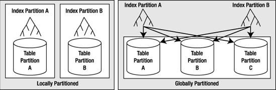
Figure 13-5. Local and global index partitions
In the case of a globally partitioned index, note that the number of index partitions may, in fact, be different from the number of table partitions.
Since global indexes may be partitioned by range or hash only, you must use local indexes if you wish to have a list or composite partitioned index. The local index will be partitioned using the same scheme as the underlying table.
Note Hash partitioning of global indexes is a new feature in Oracle 10g Release 1 and later only. You may only globally partition by range in Oracle9i and before.
Local Indexes vs. Global Indexes
In my experience, most partition implementations in data warehouse systems use local indexes. In an OLTP system, global indexes are much more common, and we'll see why shortly—it has to do with the need to perform partition elimination on the index structures to maintain the same query response times after partitioning as before partitioning them.
Note Over the last couple of years, it has become more common to see local indexes used in OLTP systems, as such systems have rapidly grown in size.
Local indexes have certain properties that make them the best choice for most data warehouse implementations. They support a more available environment (less downtime), since problems will be isolated to one range or hash of data. Since it can point to many table partitions, a global index, on the other hand, may become a point of failure, rendering all partitions inaccessible to certain queries.
Local indexes are more flexible when it comes to partition maintenance operations. If the DBA decides to move a table partition, only the associated local index partition needs to be rebuilt or maintained. With a global index, all index partitions must be rebuilt or maintained in real time. The same is true with sliding window implementations, where old data is aged out of the partition and new data is aged in. No local indexes will be in need of a rebuild, but all global indexes will be either rebuilt or maintained during the partition operation. In some cases, Oracle can take advantage of the fact that the index is locally partitioned with the table and will develop optimized query plans based on that. With global indexes, there is no such relationship between the index and table partitions.
Local indexes also facilitate a partition point-in-time recovery operation. If a single partition needs to be recovered to an earlier point in time than the rest of the table for some reason, all locally partitioned indexes can be recovered to that same point in time. All global indexes would need to be rebuilt on this object. This does not mean "avoid global indexes"—in fact, they are vitally important for performance reasons, as you'll learn shortly—you just need to be aware of the implications of using them.
Local Indexes
Oracle makes a distinction between the following two types of local indexes:
- Local prefixed indexes: These are indexes whereby the partition keys are on the leading edge of the index definition. For example, if a table is range partitioned on a column named
LOAD_DATE, a local prefixed index on that table would haveLOAD_DATEas the first column in its column list. - Local nonprefixed indexes: These indexes do not have the partition key on the leading edge of their column list. The index may or may not contain the partition key columns.
Both types of indexes are able take advantage of partition elimination, both can support uniqueness (as long as the nonprefixed index includes the partition key), and so on. The fact is that a query that uses a local prefixed index will always allow for index partition elimination, whereas a query that uses a local nonprefixed index might not. This is why local nonprefixed indexes are said to be "slower" by some people—they do not enforce partition elimination (but they do support it).
There is nothing inherently better about a local prefixed index as opposed to a local nonprefixed index when that index is used as the initial path to the table in a query. What I mean by that is that if the query can start with "scan an index" as the first step, there isn't much difference between a prefixed and a nonprefixed index.
Partition Elimination Behavior
For the query that starts with an index access, whether or not it can eliminate partitions from consideration all really depends on the predicate in your query. A small example will help demonstrate this. The following code creates a table, PARTITIONED_TABLE, that is range partitioned on a numeric column A such that values less than two will be in partition PART_1 and values less than three will be in partition PART_2:
ops$tkyte@ORA10G> CREATE TABLE partitioned_table

  2  ( a int,

  3    b int,

  4    data char(20)

  5  )

  6  PARTITION BY RANGE (a)

  7  (

  8  PARTITION part_1 VALUES LESS THAN(2) tablespace p1,

  9  PARTITION part_2 VALUES LESS THAN(3) tablespace p2

 10  )

 11  /

Table created.
We then create both a local prefixed index, LOCAL_PREFIXED, and a local nonprefixed index, LOCAL_NONPREFIXED. Note that the nonprefixed index does not have A on the leading edge of its definition, which is what makes it a nonprefixed index:
ops$tkyte@ORA10G> create index local_prefixed on partitioned_table (a,b) local;

Index created.


ops$tkyte@ORA10G> create index local_nonprefixed on partitioned_table (b) local;

Index created.
Next, we'll insert some data into one partition and gather statistics:
ops$tkyte@ORA10G> insert into partitioned_table

  2  select mod(rownum-1,2)+1, rownum, 'x'

  3    from all_objects;

48967 rows created.


ops$tkyte@ORA10G> begin

  2     dbms_stats.gather_table_stats

  3     ( user,

  4      'PARTITIONED_TABLE',

  5       cascade=>TRUE );

  6  end;

  7  /

PL/SQL procedure successfully completed.
We take offline tablespace P2, which contains the PART_2 partition for both the tables and indexes:
ops$tkyte@ORA10G> alter tablespace p2 offline;

Tablespace altered.
Taking tablespace P2 offline will prevent Oracle from accessing those specific index partitions. It will be as if we had suffered "media failure," causing them to become unavailable. Now we'll query the table to see what index partitions are needed by different queries. This first query is written to permit the use of the local prefixed index:
ops$tkyte@ORA10G> select * from partitioned_table where a = 1 and b = 1;

         A          B DATA

---------- ---------- --------------------

         1          1 x
That query succeeded, and we can see why by reviewing the explain plan. We'll use the built-in package DBMS_XPLAN to see what partitions this query accesses. The PSTART (partition start) and PSTOP (partition stop) columns in the output show us exactly what partitions this query needs to have online and available in order to succeed:
ops$tkyte@ORA10G> delete from plan_table;

4 rows deleted.


ops$tkyte@ORA10G> explain plan for

  2  select * from partitioned_table where a = 1 and b = 1;

Explained.

ops$tkyte@ORA10G> select * from table(dbms_xplan.display);


PLAN_TABLE_OUTPUT

----------------------------------------------------------------------------------

| Operation                          | Name              | Rows  | Pstart| Pstop |

----------------------------------------------------------------------------------

| SELECT STATEMENT                   |                   |     1 |       |       |

|  PARTITION RANGE SINGLE            |                   |     1 |     1 |     1 |

|   TABLE ACCESS BY LOCAL INDEX ROWID| PARTITIONED_TABLE |     1 |     1 |     1 |

|    INDEX RANGE SCAN                | LOCAL_PREFIXED    |     1 |     1 |     1 |

----------------------------------------------------------------------------------


Predicate Information (identified by operation id):

---------------------------------------------------

  3 - access("A"=1 AND "B"=1)
Note The DBMS_XPLAN output has been edited to remove information that was not relevant, in order to permit the examples to fit on the printed page.
So, the query that uses LOCAL_PREFIXED succeeds. The optimizer was able to exclude PART_2 of LOCAL_PREFIXED from consideration because we specified A=1 in the query, and we can see clearly in the plan that PSTART and PSTOP are both equal to 1. Partition elimination kicked in for us. The second query fails, however:
ops$tkyte@ORA10G> select * from partitioned_table where b = 1;

ERROR:

ORA-00376: file 13 cannot be read at this time

ORA-01110: data file 13: '/home/ora10g/.../o1_mf_p2_1dzn8jwp_.dbf'

no rows selected
And using the same technique, we can see why:
ops$tkyte@ORA10G> delete from plan_table;

4 rows deleted.


ops$tkyte@ORA10G> explain plan for

  2 select * from partitioned_table where b = 1;

Explained.


ops$tkyte@ORA10G> select * from table(dbms_xplan.display);


PLAN_TABLE_OUTPUT

----------------------------------------------------------------------------------

| Operation                          | Name              | Rows  | Pstart| Pstop |

----------------------------------------------------------------------------------

| SELECT STATEMENT                   |                   |     1 |       |       |

|  PARTITION RANGE ALL               |                   |     1 |     1 |     2 |

|   TABLE ACCESS BY LOCAL INDEX ROWID| PARTITIONED_TABLE |     1 |     1 |     2 |

|    INDEX RANGE SCAN                | LOCAL_NONPREFIXED |     1 |     1 |     2 |

----------------------------------------------------------------------------------


Predicate Information (identified by operation id):

---------------------------------------------------

  3 - access("B"=1)
Here the optimizer was not able to remove PART_2 of LOCAL_NONPREFIXED from consideration—it needed to look in both the PART_1 and PART_2 partitions of the index to see if B=1 was in there. Herein lies a performance issue with local nonprefixed indexes: they do not make you use the partition key in the predicate as a prefixed index does. It is not that prefixed indexes are better; it's just that in order to use them, you must use a query that allows for partition elimination.
If we drop the LOCAL_PREFIXED index and rerun the original successful query as follows:
ops$tkyte@ORA10G> drop index local_prefixed;

Index dropped.


ops$tkyte@ORA10G> select * from partitioned_table where a = 1 and b = 1;

         A          B DATA

---------- ---------- --------------------

         1          1 x
it succeeds, but as we'll see, it used the same index that just a moment ago failed us. The plan shows that Oracle was able to employ partition elimination here—the predicate A=1 was enough information for the database to eliminate index partition PART_2 from consideration:
ops$tkyte@ORA10G> delete from plan_table;

4 rows deleted.


ops$tkyte@ORA10G> explain plan for

  2  select * from partitioned_table where a = 1 and b = 1;

Explained.


ops$tkyte@ORA10G> select * from table(dbms_xplan.display);

PLAN_TABLE_OUTPUT

----------------------------------------------------------------------------------

| Operation                          | Name              | Rows  | Pstart| Pstop |

----------------------------------------------------------------------------------

| SELECT STATEMENT                   |                   |     1 |       |       |

|  PARTITION RANGE SINGLE            |                   |     1 |     1 |     1 |

|   TABLE ACCESS BY LOCAL INDEX ROWID| PARTITIONED_TABLE |     1 |     1 |     1 |

|    INDEX RANGE SCAN                | LOCAL_NONPREFIXED |     1 |     1 |     1 |

----------------------------------------------------------------------------------


Predicate Information (identified by operation id):

---------------------------------------------------

   2 - filter("A"=1)

   3 - access("B"=1)
Note the PSTART and PSTOP column values of 1 and 1.This proves that the optimizer is able to perform partition elimination even for nonprefixed local indexes.
If you frequently query the preceding table with the following queries:
select ... from partitioned_table where a = :a and b = :b;

select ... from partitioned_table where b = :b;
then you might consider using a local nonprefixed index on (b,a). That index would be useful for both of the preceding queries. The local prefixed index on (a,b) would be useful only for the first query.
The bottom line here is that you should not be afraid of nonprefixed indexes or consider them to be major performance inhibitors. If you have many queries that could benefit from a nonprefixed index as outlined previously, then you should consider using one. The main concern is to ensure that your queries contain predicates that allow for index partition elimination whenever possible. The use of prefixed local indexes enforces that consideration. The use of nonprefixed indexes does not. Consider also how the index will be used. If it will be used as the first step in a query plan, there are not many differences between the two types of indexes.
Local Indexes and Unique Constraints
To enforce uniqueness—and that includes a UNIQUE constraint or PRIMARY KEY constraints—your partitioning key must be included in the constraint itself if you want to use a local index to enforce the constraint. This is the largest limitation of a local index, in my opinion. Oracle enforces uniqueness only within an index partition—never across partitions. What this implies, for example, is that you cannot range partition on a TIMESTAMP field and have a primary key on the ID that is enforced using a locally partitioned index. Oracle will instead utilize a global index to enforce uniqueness.
In the next example, we will create a range partitioned table that is partitioned by a column named LOAD_TYPE, but has a primary key on the ID column. We can do that by executing the following CREATE TABLE statement in a schema that owns no other objects, so we can easily see exactly what objects are created by looking at every segment this user owns:
ops$tkyte@ORA10G> CREATE TABLE partitioned

  2  ( load_date date,

  3    id        int,

  4    constraint partitioned_pk primary key(id)

  5  )

  6  PARTITION BY RANGE (load_date)

  7  (

  8  PARTITION part_1 VALUES LESS THAN

  9  ( to_date('01/01/2000','dd/mm/yyyy') ),

 10  PARTITION part_2 VALUES LESS THAN

 11  ( to_date('01/01/2001','dd/mm/yyyy') )

 12  )

 13  /

Table created.


ops$tkyte@ORA10G> select segment_name, partition_name, segment_type

  2    from user_segments;


SEGMENT_NAME   PARTITION_NAME  SEGMENT_TYPE

-------------- --------------- ------------------

PARTITIONED    PART_1          TABLE PARTITION

PARTITIONED    PART_2          TABLE PARTITION

PARTITIONED_PK                 INDEX
The PARTITIONED_PK index is not even partitioned, let alone locally partitioned, and as we'll see, it cannot be locally partitioned. Even if we try to trick Oracle by realizing that a primary key can be enforced by a nonunique index as well as a unique index, we'll find that this approach will not work either:
ops$tkyte@ORA10G> CREATE TABLE partitioned

  2  ( timestamp date,

  3    id        int

  4  )

  5  PARTITION BY RANGE (timestamp)

  6  (

  7  PARTITION part_1 VALUES LESS THAN

  8  ( to_date('01-jan-2000','dd-mon-yyyy') ),

  9  PARTITION part_2 VALUES LESS THAN

 10  ( to_date('01-jan-2001','dd-mon-yyyy') )

 11  )

 12  /

Table created.


ops$tkyte@ORA10G> create index partitioned_idx

  2  on partitioned(id) local

  3  /

Index created.


ops$tkyte@ORA10G> select segment_name, partition_name, segment_type

  2    from user_segments;


SEGMENT_NAME     PARTITION_NAME SEGMENT_TYPE

--------------- --------------- ------------------

PARTITIONED     PART_1          TABLE PARTITION

PARTITIONED_IDX PART_2          INDEX PARTITION

PARTITIONED     PART_2          TABLE PARTITION

PARTITIONED_IDX PART_1          INDEX PARTITION


ops$tkyte@ORA10G> alter table partitioned

  2  add constraint

  3  partitioned_pk

  4  primary key(id)

  5  /

alter table partitioned

*

ERROR at line 1:

ORA-01408: such column list already indexed
Here, Oracle attempts to create a global index on ID, but finds that it cannot since an index already exists. The preceding statements would work if the index we created was not partitioned, as Oracle would have used that index to enforce the constraint.
The reasons why uniqueness cannot be enforced, unless the partition key is part of the constraint, are twofold. First, if Oracle allowed this, it would void most of the advantages of partitions. Availability and scalability would be lost, as each and every partition would always have to be available and scanned to do any inserts and updates. The more partitions you had, the less available the data would be. The more partitions you had, the more index partitions you would have to scan, and the less scalable partitions would become. Instead of providing availability and scalability, doing this would actually decrease both.
Additionally, Oracle would have to effectively serialize inserts and updates to this table at the transaction level. This is because if we add ID=1 to PART_1, Oracle would have to somehow prevent anyone else from adding ID=1 to PART_2. The only way to do this would be to prevent others from modifying index partition PART_2, since there isn't anything to really "lock" in that partition.
In an OLTP system, unique constraints must be system enforced (i.e., enforced by Oracle) to ensure the integrity of data. This implies that the logical model of your application will have an impact on the physical design. Uniqueness constraints will either drive the underlying table partitioning scheme, driving the choice of the partition keys, or point you toward the use of global indexes instead. We'll take a look at global indexes in more depth next.
Global Indexes
Global indexes are partitioned using a scheme that is different from that used in the underlying table. The table might be partitioned by a TIMESTAMP column into ten partitions, and a global index on that table could be partitioned into five partitions by the REGION column. Unlike local indexes, there is only one class of global index, and that is a prefixed global index. There is no support for a global index whose index key does not begin with the partitioning key for that index. That implies that whatever attribute(s) you use to partition the index will be on the leading edge of the index key itself.
Continuing on from our previous example, here is a quick example of the use of a global index. It shows that a global partitioned index can be used to enforce uniqueness for a primary key, so you can have partitioned indexes that enforce uniqueness, but do not include the partition key of TABLE. The following example creates a table partitioned by TIMESTAMP that has an index partitioned by ID:
ops$tkyte@ORA10G> CREATE TABLE partitioned

  2  ( timestamp date,

  3    id        int

  4  )

  5  PARTITION BY RANGE (timestamp)

  6  (

  7  PARTITION part_1 VALUES LESS THAN

  8  ( to_date('01-jan-2000','dd-mon-yyyy') ),

  9  PARTITION part_2 VALUES LESS THAN

 10  ( to_date('01-jan-2001','dd-mon-yyyy') )

 11  )

 12  /

Table created.


ops$tkyte@ORA10G> create index partitioned_index

  2  on partitioned(id)

  3  GLOBAL

  4  partition by range(id)

  5  (

  6  partition part_1 values less than(1000),

  7  partition part_2 values less than (MAXVALUE)

  8  )

  9  /

Index created.
Note the use of MAXVALUE in this index. MAXVALUE can be used in any range partitioned table as well as in the index. It represents an "infinite upper bound" on the range. In our examples so far, we've used hard upper bounds on the ranges (values less than <some value>). However, a global index has a requirement that the highest partition (the last partition) must have a partition bound whose value is MAXVALUE. This ensures that all rows in the underlying table can be placed in the index.
Now, completing this example, we'll add our primary key to the table:
ops$tkyte@ORA10G> alter table partitioned add constraint

  2  partitioned_pk

  3  primary key(id)

  4  /

Table altered.
It is not evident from this code that Oracle is using the index we created to enforce the primary key (it is to me because I know that Oracle is using it), so we can prove it by simply trying to drop that index:
ops$tkyte@ORA10G> drop index partitioned_index;

drop index partitioned_index

           *

ERROR at line 1:

ORA-02429: cannot drop index used for enforcement of unique/primary key
To show that Oracle will not allow us to create a nonprefixed global index, we only need try the following:
ops$tkyte@ORA10G> create index partitioned_index2

  2  on partitioned(timestamp,id)

  3  GLOBAL

  4  partition by range(id)

  5  (

  6  partition part_1 values less than(1000),

  7  partition part_2 values less than (MAXVALUE)

  8  )

  9  /

partition by range(id)

           *

ERROR at line 4:

ORA-14038: GLOBAL partitioned index must be prefixed
The error message is pretty clear. The global index must be prefixed. So, when would you use a global index? We'll take a look at two system types, data warehouse and OLTP, and see when they might apply.
Data Warehousing and Global Indexes
In the past, it used to be that data warehousing and global indexes were pretty much mutually exclusive. A data warehouse implies certain things, such as large amounts of data coming in and going out. Many data warehouses implement a sliding window approach to managing data—that is, drop the oldest partition of a table and add a new partition for the newly loaded data. In the past (Oracle8i and earlier), these systems would have avoided the use of global indexes for a very good reason: lack of availability. It used to be the case that most partition operations, such as dropping an old partition, would invalidate the global indexes, rendering them unusable until they were rebuilt. This could seriously compromise availability.
In the following sections, we'll take a look at what is meant by a sliding window of data and the potential impact of a global index on it. I stress the word "potential" because we'll also look at how we may get around this issue and how to understand what getting around the issue might imply.
Sliding Windows and Indexes
The following example implements a classic sliding window of data. In many implementations, data is added to a warehouse over time and the oldest data is aged out. Many times, this data is range partitioned by a date attribute, so that the oldest data is stored together in a single partition, and the newly loaded data is likewise stored together in a new partition. The monthly load process involves
- Detaching the old data: The oldest partition is either dropped or exchanged with an empty table (turning the oldest partition into a table) to permit archiving of the old data.
- Loading and indexing of the new data: The new data is loaded into a "work" table and indexed and validated.
- Attaching the new data: Once the new data is loaded and processed, the table it is in is exchanged with an empty partition in the partitioned table, turning this newly loaded data in a table into a partition of the larger partitioned table.
This process is repeated every month, or however often the load process is performed; it could be every day or every week. We will implement this very typical process in this section to show the impact of global partitioned indexes and demonstrate the options we have during partition operations to increase availability, allowing us to implement a sliding window of data and maintain continuous availability of data.
We'll process yearly data in this example and have fiscal years 2004 and 2005 loaded up. The table will be partitioned by the TIMESTAMP column, and it will have two indexes created on it—one is a locally partitioned index on the ID column, and the other is a global index (nonpartitioned, in this case) on the TIMESTAMP column:
ops$tkyte@ORA10G> CREATE TABLE partitioned

  2  ( timestamp date,

  3    id        int

  4  )

  5  PARTITION BY RANGE (timestamp)

  6  (

  7  PARTITION fy_2004 VALUES LESS THAN

  8  ( to_date('01-jan-2005','dd-mon-yyyy') ),

  9  PARTITION fy_2005 VALUES LESS THAN

 10  ( to_date('01-jan-2006','dd-mon-yyyy') )

 11  )

 12  /

Table created.


ops$tkyte@ORA10G> insert into partitioned partition(fy_2004)

  2  select to_date('31-dec-2004','dd-mon-yyyy')-mod(rownum,360), object_id

  3  from all_objects

  4  /

48514 rows created.


ops$tkyte@ORA10G> insert into partitioned partition(fy_2005)

  2  select to_date('31-dec-2005','dd-mon-yyyy')-mod(rownum,360), object_id

  3  from all_objects

  4  /

48514 rows created.


ops$tkyte@ORA10G> create index partitioned_idx_local

  2  on partitioned(id)

  3  LOCAL

  4  /

Index created.


ops$tkyte@ORA10G> create index partitioned_idx_global

  2  on partitioned(timestamp)

  3  GLOBAL

  4  /

Index created.
This sets up our "warehouse" table. The data is partitioned by fiscal year and we have the last two years' worth of data online. This table has two indexes: one is LOCAL and the other is GLOBAL. Now it is the end of the year and we would like to do the following:
- Remove the oldest fiscal year data. We do not want to lose this data forever; we just want to age it out and archive it.
- Add the newest fiscal year data. It will take a while to load it, transform it, index it, and so on. We would like to do this work without impacting the availability of the current data, if at all possible.
The first step we might take would be to set up an empty table for fiscal year 2004 that looks just like the partitioned table. We'll use this table to exchange with the FY_2004 partition in the partitioned table, turning that partition into a table and in turn emptying out the partition in the partitioned table. The net effect is that the oldest data in the partitioned table will have been, in effect, removed after the exchange:
ops$tkyte@ORA10G> create table fy_2004 ( timestamp date, id int );

Table created.


ops$tkyte@ORA10G> create index fy_2004_idx on fy_2004(id)

  2  /

Index created.
We'll do the same to the new data to be loaded. We'll create and load a table that structurally looks like the existing partitioned table (but that is not itself partitioned):
ops$tkyte@ORA10G> create table fy_2006 ( timestamp date, id int );

Table created.


ops$tkyte@ORA10G> insert into fy_2006

  2  select to_date('31-dec-2006','dd-mon-yyyy')-mod(rownum,360), object_id

  3  from all_objects

  4  /

48521 rows created.


ops$tkyte@ORA10G> create index fy_2006_idx on fy_2006(id) nologging

  2  /

Index created.
We'll turn the current full partition into an empty partition and create a "full" table, with the FY_2004 data in it. Also, we've completed all of the work necessary to have the FY_2006 data ready to go. This would have involved verifying the data, transforming it—whatever complex tasks we need to undertake to get it ready.
Now we're ready to update the "live" data using an exchange partition:
ops$tkyte@ORA10G> alter table partitioned

  2  exchange partition fy_2004

  3  with table fy_2004

  4  including indexes

  5  without validation

  6  /

Table altered.


ops$tkyte@ORA10G> alter table partitioned

  2  drop partition fy_2004

  3  /

Table altered.
This is all we need to do to "age" the old data out. We turned the partition into a full table and the empty table into a partition. This was a simple data dictionary update. No large amount of I/O took place—it just happened. We can now export that FY_2004 table (perhaps using a transportable tablespace) out of our database for archival purposes. We could reattach it quickly if we ever needed to.
Next, we want to slide in the new data:
ops$tkyte@ORA10G> alter table partitioned

  2  add partition fy_2006

  3  values less than ( to_date('01-jan-2007','dd-mon-yyyy') )

  4  /

Table altered.


ops$tkyte@ORA10G> alter table partitioned

  2  exchange partition fy_2006

  3  with table fy_2006

  4  including indexes

  5  without validation

  6  /

Table altered.
Again, this was instantaneous; it was accomplished via simple data dictionary updates. Adding the empty partition took very little time to process. Then, we exchange the newly created empty partition with the full table, and the full table with the empty partition, and that operation is performed quickly as well. The new data is online.
Looking at our indexes, however, we'll find the following:
ops$tkyte@ORA10G> select index_name, status from user_indexes;


INDEX_NAME                     STATUS

------------------------------ --------

FY_2006_IDX                    VALID

FY_2004_IDX                    VALID

PARTITIONED_IDX_GLOBAL         UNUSABLE

PARTITIONED_IDX_LOCAL          N/A
The global index is, of course, unusable after this operation. Since each index partition can point to any table partition, and we just took away a partition and added a partition, that index is invalid. It has entries that point into the partition we dropped. It has no entries that point into the partition we just added. Any query that would make use of this index either will fail and not execute or, if we skip unusable indexes, the query's performance will be negatively impacted by not being able to use the index:
ops$tkyte@ORA10G> set autotrace on explain

ops$tkyte@ORA10G> select /*+ index( partitioned PARTITIONED_IDX_GLOBAL ) */ count(*)

  2  from partitioned

  3  where timestamp between sysdate-50 and sysdate;

select /*+ index( partitioned PARTITIONED_IDX_GLOBAL ) */ count(*)

*

ERROR at line 1:

ORA-01502: index 'OPS$TKYTE.PARTITIONED_IDX_GLOBAL' or partition

           of such index is in unusable state


ops$tkyte@ORA10G> select count(*)

  2  from partitioned

  3  where timestamp between sysdate-50 and sysdate;


  COUNT(*)

----------

      6750


Execution Plan

----------------------------------------------------------

  0       SELECT STATEMENT Optimizer=ALL_ROWS (Cost=59 Card=1 Bytes=9)

  1     0   SORT (AGGREGATE)

  2     1     FILTER

  3     2       PARTITION RANGE (ITERATOR) (Cost=59 Card=7234 Bytes=65106)

  4     3         TABLE ACCESS (FULL) OF 'PARTITIONED' (TABLE) (Cost=59 Card=7234


ops$tkyte@ORA10G> set autotrace off
So, our choices after performing this partition operation with global indexes are
- Skip the index, either transparently as Oracle 10g is doing in this example or by setting the session parameter
SKIP_UNUSABLE_INDEXES=TRUEin 9i (Oracle 10g defaults this setting toTRUE). But then we lose the performance the index was giving us. - Have the query receive an error, as it would in 9i unless
SKIP_UNUSABLE_INDEXESwere set toFALSE, and as would any query in 10g that explicitly requests to use a hint. We need to rebuild this index to make the data truly usable again.
The sliding window process, which so far has resulted in virtually no downtime, will now take a very long time to complete while we rebuild the global index. Runtime query performance of queries that relied on these indexes will be negatively affected during this time—either they will not run at all or they will run without the benefit of the index. All of the data must be scanned and the entire index reconstructed from the table data. If the table is many hundreds of gigabytes in size, this will take considerable resources.
"Live" Global Index Maintenance
Starting in Oracle9i, another option was added to partition maintenance: the ability to maintain the global indexes during the partition operation using the UPDATE GLOBAL INDEXES clause. This means that as you drop a partition, split a partition, perform whatever operation necessary on a partition, Oracle will perform the necessary modifications to the global index to keep it up to date. Since most partition operations will cause this global index invalidation to occur, this feature can be a boon to systems that need to provide continual access to the data. You'll find that you sacrifice the raw speed of the partition operation, but with the associated window of unavailability immediately afterward as you rebuild indexes, for a slower overall response time from the partition operation but coupled with 100 percent data availability. In short, if you have a data warehouse that cannot have downtime, but must support these common data warehouse techniques of sliding data in and out, then this feature is for you—but you must understand the implications.
Revisiting our previous example, if our partition operations had used the UPDATE GLOBAL INDEXES clause when relevant (in this example, it would not be needed on the ADD PARTITION statement since the newly added partition would not have any rows in it),
ops$tkyte@ORA10G> alter table partitioned

  2  exchange partition fy_2004

  3  with table fy_2004

  4  including indexes

  5  without validation

  6  UPDATE GLOBAL INDEXES

  7  /

Table altered.


ops$tkyte@ORA10G> alter table partitioned

  2  drop partition fy_2004

  3  UPDATE GLOBAL INDEXES

  4  /

Table altered.


ops$tkyte@ORA10G> alter table partitioned

  2  add partition fy_2006

  3  values less than ( to_date('01-jan-2007','dd-mon-yyyy') )

  4  /

Table altered.


ops$tkyte@ORA10G> alter table partitioned

  2  exchange partition fy_2006

  3  with table fy_2006

  4  including indexes

  5  without validation

  6  UPDATE GLOBAL INDEXES

  7  /

Table altered.
then we would have discovered the indexes to be perfectly valid and usable both during and after the operation:
ops$tkyte@ORA10G> select index_name, status from user_indexes;


INDEX_NAME                     STATUS

------------------------------ --------

FY_2006_IDX                    VALID

FY_2004_IDX                    VALID

PARTITIONED_IDX_GLOBAL         VALID

PARTITIONED_IDX_LOCAL          N/A


6  rows selected.


ops$tkyte@ORA10G> set autotrace on explain

ops$tkyte@ORA10G> select count(*)

  2  from partitioned

  3  where timestamp between sysdate-50 and sysdate;


  COUNT(*)

----------

      6750


Execution Plan

----------------------------------------------------------

  0       SELECT STATEMENT Optimizer=ALL_ROWS (Cost=9 Card=1 Bytes=9)

  1     0   SORT (AGGREGATE)

  2     1     FILTER

  3     2       INDEX (RANGE SCAN) OF 'PARTITIONED_IDX_GLOBAL' (INDEX) (Cost=9...
But there is a tradeoff: we are performing the logical equivalent of INSERT and DELETE operations on the global index structures. When we drop a partition, we have to delete all of the global index entries that might be pointing to that partition. When we did the exchange of a table with a partition, we had to delete all of the global index entries pointing to the original data and then insert all of the new ones that we just slid in there. So the amount of work performed by the ALTER commands was significantly increased.
In fact, using runstats and a slightly modified version of the preceding example, we can measure the amount of "extra" work performed to maintain the global indexes during the partition operation. We'll slide out FY_2004 and slide in FY_2006 as before, adding in the requisite index rebuild. This will be the sliding window implementation that causes the data to become unavailable due to the need to rebuild the global indexes. We'll also then slide out FY_2005 and slide in FY_2007 using the UPDATE GLOBAL INDEXES clause, to emulate the sliding window implementation that provides for full data availability, even during the partition operations. In that manner, we can measure the same operations using the different techniques and compare them. Our expected outcome will be that the first approach will consume fewer database resources and, therefore, perform "faster" but will incur a measurable period of "downtime." The second approach, while consuming more resources and perhaps taking longer overall, will not incur downtime. As far as the end users are concerned, their ability to work never ceased. They might have been processing a bit slower (since we were competing with them for resources), but they were still processing, and they never stopped.
So, if we take the earlier example, but also create an empty FY_2005 table like FY_2004, and a full FY_2007 table like FY_2006, we can measure the differences between the index rebuild approaches, starting first with the "less available approach":
exec runStats_pkg.rs_start;


alter table partitioned exchange partition fy_2004

with table fy_2004 including indexes without validation;


alter table partitioned drop partition fy_2004;


alter table partitioned add partition fy_2006

values less than ( to_date('01-jan-2007','dd-mon-yyyy') );


alter table partitioned exchange partition fy_2006

with table fy_2006 including indexes without validation;


alter index partitioned_idx_global rebuild;


exec runStats_pkg.rs_middle;
Here is the highly available UPDATE GLOBAL INDEXES approach:
alter table partitioned exchange partition fy_2005

with table fy_2005 including indexes without validation

update global indexes;


alter table partitioned drop partition fy_2005

update global indexes;


alter table partitioned add partition fy_2007

values less than ( to_date('01-jan-2008','dd-mon-yyyy') );


alter table partitioned exchange partition fy_2007

with table fy_2007 including indexes without validation

update global indexes;


exec runStats_pkg.rs_stop;
We might observe the following:
ops$tkyte@ORA10G> exec runStats_pkg.rs_stop;

Run1 ran in 81 hsecs

Run2 ran in 94 hsecs

run 1 ran in 86.17% of the time


Name                                  Run1        Run2        Diff

...

STAT...CPU used when call star          39          59          20

...

STAT...redo entries                    938       3,340       2,402

STAT...db block gets                 1,348       5,441       4,093

STAT...session logical reads         2,178       6,455       4,277

...

LATCH.cache buffers chains           5,675      27,695      22,020

...

STAT...table scan rows gotten       97,711     131,427      33,716

STAT...undo change vector size      35,100   3,404,056   3,368,956

STAT...redo size                 2,694,172   6,197,988   3,503,816
The index rebuild approach did run faster, both as observed by the elapsed time and the CPU time. This fact has caused many a DBA to pause and say, "Hey, I don't want to use UPDATE GLOBAL INDEXES—it's slower." That is too simplistic of a view, however. What you need to remember is that while the operations overall took longer, processing on your system was not necessarily interrupted. Sure, you as the DBA might be looking at your screen for a longer period of time, but the really important work that takes place on your system was still taking place. What you need to do is see if this tradeoff makes sense for you. If you have an eight-hour maintenance window overnight in which to load new data, then by all means, use the rebuild approach if that makes sense. However, if you have a mandate to be available continuously, then the ability to maintain the global indexes will be crucial.
Looking at the redo generated by each approach, we can see that the UPDATE GLOBAL INDEXES generated considerably more—over 230 percent more—and we would expect that to only go up as we add more and more global indexes to the table. The redo generated by the UPDATE GLOBAL INDEXES is unavoidable and cannot be turned off via NOLOGGING, since the maintenance of the global indexes is not a complete rebuild of their structure but more of an incremental "maintenance." Additionally, since we are maintaining the live index structure, we must generate undo for that—in the event the partition operation fails, we must be prepared to put the index back the way it was. And remember, undo is protected by redo itself, so some of the redo you see generated is from the index updates and some is from the rollback. Add another global index or two and you would reasonably expect these numbers to increase.
So, UPDATE GLOBAL INDEXES is an option that allows you to trade off availability for resource consumption. If you have the need to provide continuous availability, it will be the option for you. But you will have to understand the ramifications and size other components of your system appropriately. Specifically, many data warehouses have been crafted over time to use bulk, direct path operations, bypassing undo generation and, when permitted, redo generation as well. Using UPDATE GLOBAL INDEXES cannot bypass either of those two elements. You'll need to examine the rules you used to size these components before using this feature, so you can assure yourself it can work on your system.
An OLTP system is characterized by the frequent occurrence of many small read and write transactions. In general, fast access to the row (or rows) you need is paramount. Data integrity is vital. Availability is also very important.
Global indexes make sense in many cases in OLTP systems. Table data can be partitioned by only one key—one set of columns. However, you may need to access the data in many different ways. You might partition EMPLOYEE data by LOCATION in the table, but you still need fast access to EMPLOYEE data by
DEPARTMENT: Departments are geographically dispersed. There is no relationship between a department and a location.EMPLOYEE_ID: While an employee ID will determine a location, you don't want to have to search byEMPLOYEE_IDandLOCATION, hence partition elimination cannot take place on the index partitions. Also,EMPLOYEE_IDby itself must be unique.JOB_TITLE: There is no relationship betweenJOB_TITLEandLOCATION. AllJOB_TITLEvalues may appear in anyLOCATION.
There is a need to access the EMPLOYEE data by many different keys in different places in the application, and speed is paramount. In a data warehouse, we might just use locally partitioned indexes on these keys and use parallel index range scans to collect a large amount of data fast. In these cases, we don't necessarily need to use index partition elimination. In an OLTP system, however, we do need to use it. Parallel query is not appropriate for these systems; we need to provide the indexes appropriately. Therefore, we will need to make use of global indexes on certain fields.
The goals we need to meet are
- Fast access
- Data integrity
- Availability
Global indexes can accomplish these goals in an OLTP system. We will probably not be doing sliding windows, auditing aside for a moment. We will not be splitting partitions (unless we have a scheduled downtime), we will not be moving data, and so on. The operations we perform in a data warehouse are not done on a live OLTP system in general.
Here is a small example that shows how we can achieve the three goals just listed with global indexes. I am going to use simple, "single partition" global indexes, but the results would not be different with global indexes in multiple partitions (except for the fact that availability and manageability would increase as we added index partitions). We start with a table that is range partitioned by location, LOC, according to our rules, which places all LOC values less than 'C' into partition P1, those less than 'D' into partition P2, and so on:
ops$tkyte@ORA10G> create table emp

  2  (EMPNO             NUMBER(4) NOT NULL,

  3   ENAME             VARCHAR2(10),

  4   JOB               VARCHAR2(9),

  5   MGR               NUMBER(4),

  6   HIREDATE          DATE,

  7   SAL               NUMBER(7,2),

  8   COMM              NUMBER(7,2),

  9   DEPTNO            NUMBER(2) NOT NULL,

 10   LOC               VARCHAR2(13) NOT NULL

 11  )

 12  partition by range(loc)

 13  (

 14  partition p1 values less than('C') tablespace p1,

 15  partition p2 values less than('D') tablespace p2,

 16  partition p3 values less than('N') tablespace p3,

 17  partition p4 values less than('Z') tablespace p4

 18  )

 19  /

Table created.
We alter the table to add a constraint on the primary key column:
ops$tkyte@ORA10G> alter table emp add constraint emp_pk

  2  primary key(empno)

  3  /

Table altered.
A side effect of this is that there exists a unique index on the EMPNO column. This shows we can support and enforce data integrity, one of our goals. Finally, we create two more global indexes on DEPTNO and JOB, to facilitate accessing records quickly by those attributes:
ops$tkyte@ORA10G> create index emp_job_idx on emp(job)

  2  GLOBAL

  3  /

Index created.


ops$tkyte@ORA10G> create index emp_dept_idx on emp(deptno)

  2  GLOBAL

  3  /

Index created.


ops$tkyte@ORA10G> insert into emp

  2  select e.*, d.loc

  3   from scott.emp e, scott.dept d

  4  where e.deptno = d.deptno

  5  /

14 rows created.
Now let's see what is in each partition:
ops$tkyte@ORA10G> break on pname skip 1

ops$tkyte@ORA10G> select 'p1' pname, empno, job, loc from emp partition(p1)

  2  union all

  3  select 'p2' pname, empno, job, loc from emp partition(p2)

  4  union all

  5  select 'p3' pname, empno, job, loc from emp partition(p3)

  6  union all

  7  select 'p4' pname, empno, job, loc from emp partition(p4)

  8  /


PN      EMPNO JOB       LOC

-- ---------- --------- -------------

p2       7499 SALESMAN  CHICAGO

         7698 MANAGER   CHICAGO

         7654 SALESMAN  CHICAGO

         7900 CLERK     CHICAGO

         7844 SALESMAN  CHICAGO

         7521 SALESMAN  CHICAGO


p3       7369 CLERK     DALLAS

         7876 CLERK     DALLAS

         7902 ANALYST   DALLAS

         7788 ANALYST   DALLAS

         7566 MANAGER   DALLAS


p4       7782 MANAGER   NEW YORK

         7839 PRESIDENT NEW YORK

         7934 CLERK     NEW YORK

14 rows selected.
This shows the distribution of data, by location, into the individual partitions. We can now review some query plans to see what we could expect performance-wise:
ops$tkyte@ORA10G> variable x varchar2(30);

ops$tkyte@ORA10G> begin

  2     dbms_stats.set_table_stats

  3     ( user, 'EMP', numrows=>100000, numblks => 10000 );

  4  end;

  5  /

PL/SQL procedure successfully completed.


ops$tkyte@ORA10G> delete from plan_table;

3 rows deleted.


ops$tkyte@ORA10G> explain plan for

  2  select empno, job, loc from emp where empno = :x;

Explained.


ops$tkyte@ORA10G> select * from table(dbms_xplan.display);


PLAN_TABLE_OUTPUT

------------------------------------------------------------------------

| Operation                          | Name   |Rows |Bytes|Pstart|Pstop|

------------------------------------------------------------------------

| SELECT STATEMENT                   |        |    1|   27|      |     |

|  TABLE ACCESS BY GLOBAL INDEX ROWID| EMP    |    1|   27|ROWID |ROWID|

|   INDEX UNIQUE SCAN                | EMP_PK |    1|     |      |     |

------------------------------------------------------------------------

Predicate Information (identified by operation id):

---------------------------------------------------

  2 - access("EMPNO"=TO_NUMBER(:X))
Note The explain plan format has been edited to fit on the page. Columns in the report not relevant to the discussion have been omitted.
The plan here shows an INDEX UNIQUE SCAN of the nonpartitioned index EMP_PK that was created in support of our primary key. Then there is a TABLE ACCESS BY GLOBAL INDEX ROWID, with a PSTART and PSTOP of ROWID/ROWID, meaning that when we get the ROWID from the index, it will tell us precisely which index partition to read to get this row. This index access will be as effective as on a nonpartitioned table and perform the same amount of I/O to do so. It is just a simple, single index unique scan followed by a "get this row by ROWID." Now, let's look at one of the other global indexes, the one on JOB:
ops$tkyte@ORA10G> delete from plan_table;

3 rows deleted.


ops$tkyte@ORA10G> explain plan for

  2 select  empno, job, loc from emp where job = :x;

Explained.


ops$tkyte@ORA10G> select * from table(dbms_xplan.display);


PLAN_TABLE_OUTPUT

---------------------------------------------------------------------------

| Operation                          |Name       |Rows |Bytes|Pstart|Pstop|

---------------------------------------------------------------------------

| SELECT STATEMENT                   |           | 1000|27000|      |     |

|  TABLE ACCESS BY GLOBAL INDEX ROWID|EMP        | 1000|27000|ROWID |ROWID|

|   INDEX RANGE SCAN                 |EMP_JOB_IDX|  400|     |      |     |

---------------------------------------------------------------------------

Predicate Information (identified by operation id):

---------------------------------------------------

  2 - access("JOB"=:X)
Sure enough, we see a similar effect for the INDEX RANGE SCAN. Our indexes are used and can provide high-speed OLTP access to the underlying data. If they were partitioned, they would have to be prefixed and enforce index partition elimination; hence, they are scalable as well, meaning we can partition them and observe the same behavior. In a moment, we'll look at what would happen if we used LOCAL indexes only.
Lastly, let's look at the area of availability. The Oracle documentation claims that globally partitioned indexes make for "less available" data than locally partitioned indexes. I don't fully agree with this blanket characterization. I believe that in an OLTP system they are as highly available as a locally partitioned index. Consider the following:
ops$tkyte@ORA10G> alter tablespace p1 offline;

Tablespace altered.


ops$tkyte@ORA10G> alter tablespace p2 offline;

Tablespace altered.


ops$tkyte@ORA10G> alter tablespace p3 offline;

Tablespace altered.


ops$tkyte@ORA10G> select empno, job, loc from emp where empno = 7782;


     EMPNO JOB       LOC

---------- --------- -------------

     7782  MANAGER   NEW YORK
Here, even though most of the underlying data is unavailable in the table, we can still gain access to any bit of data available via that index. As long as the EMPNO we want is in a tablespace that is available, and our GLOBAL index is available, our GLOBAL index works for us. On the other hand, if we had been using the "highly available" local index in the preceding case, we might have been prevented from accessing the data! This is a side effect of the fact that we partitioned on LOC but needed to query by EMPNO. We would have had to probe each local index partition and would have failed on the index partitions that were not available.
Other types of queries, however, will not (and cannot) function at this point in time:
ops$tkyte@ORA10G> select empno, job, loc from emp where job = 'CLERK';

select empno, job, loc from emp where job = 'CLERK'

                            *

ERROR at line 1:

ORA-00376: file 13 cannot be read at this time

ORA-01110: data file 13: '/home/ora10g/oradata/.../o1_mf_p2_1dzn8jwp_.dbf'
The CLERK data is in all of the partitions, and the fact that three of the tablespaces are offline does affect us. This is unavoidable unless we had partitioned on JOB, but then we would have had the same issues with queries that needed data by LOC. Anytime you need to access the data from many different "keys," you will have this issue. Oracle will give you the data whenever it can.
Note, however, that if the query can be answered from the index, avoiding the TABLE ACCESS BY ROWID, the fact that the data is unavailable is not as meaningful:
ops$tkyte@ORA10G> select count(*) from emp where job = 'CLERK';


   COUNT(*)

----------

         4
Since Oracle didn't need the table in this case, the fact that most of the partitions were offline doesn't affect this query. As this type of optimization (i.e., answer the query using just the index) is common in an OLTP system, there will be many applications that are not affected by the data that is offline. All we need to do now is make the offline data available as fast as possible (restore it and recover it).
Partitioning and Performance, Revisited
Many times I hear people say, "I'm very disappointed in partitioning. We partitioned our largest table and it went much slower. So much for partitioning being a performance increasing feature."
Partitioning can do one of the following three things to overall query performance:
- Make your queries go faster
- Not impact the performance of your queries at all
- Make your queries go much slower and use many times the resources as the nonpartitioned implementation
In a data warehouse, with an understanding of the questions being asked of the data, the first bullet point is very much achievable. Partitioning can positively impact queries that frequently full scan large database tables by eliminating large sections of data from consideration. Suppose you have a table with 1 billion rows in it. There is a timestamp attribute. Your query is going to retrieve one years' worth of data from this table (and it has ten years of data). Your query uses a full table scan to retrieve this data. Had it been partitioned by this timestamp entry—say, a partition per month—then you could have full scanned one-tenth the data (assuming a uniform distribution of data over the years). Partition elimination would have removed the other 90 percent of the data from consideration. Your query would likely run faster.
Now, take a similar table in an OLTP system. You would never retrieve 10 percent of a 1 billion row table in that type of application. Therefore, the massive increase in speed seen by the data warehouse just would not be achievable in a transactional system. You are not doing the same sort of work, and the same possible improvements just are not realistic. Therefore, in general, in your OLTP system the first bullet point is not achievable, and you won't be applying partitioning predominantly for increased performance. Increased availability—absolutely. Administrative ease of use—very much so. But in an OLTP system, I say you have to work hard to make sure you achieve the second point: that you do not impact the performance of your queries at all, negatively or positively. Many times, your goal is to apply partitioning without affecting query response time.
On many occasions, I've seen that the implementation team will see they have a large table, say of 10 million rows. Now, 10 million sounds like an incredibly large number (and five or ten years ago, it would have been, but time changes all things). The team decides to partition the data. But in looking at the data, there are no logical attributes that make sense for RANGE partitioning. There are no sensible attributes for that. Likewise, LIST partitioning doesn't make sense. Nothing pops out of this table as being the "right thing" to partition by. So, the team opts for hash partitioning on the primary key, which just happens to be populated by an Oracle sequence number. It looks perfect, it is unique and easy to hash, and many queries are of the form SELECT * FROM T WHERE PRIMARY_KEY = :X.
But the problem is, there are many other queries against this object that are not of that form. For illustrative purposes, assume the table in question is really the ALL_OBJECTS dictionary view, and while internally many queries would be of the form WHERE OBJECT_ID = :X, the end users frequently have these requests of the application as well:
- Show me the details of
SCOTT's EMP TABLE (WHERE OWNER = :O AND OBJECT_TYPE = :T). AND OBJECT_NAME = :N
 - Show me all of the tables
SCOTTowns (WHERE OWNER = :O AND OBJECT_TYPE = :T). - Show me all of the objects
SCOTTowns (WHERE OWNER = :O).
In support of those queries, you have an index on (OWNER,OBJECT_TYPE,OBJECT_NAME). But you also read that "local indexes are more available," and you would like to be more available regarding your system, so you implement with them. You end up re-creating your table like this, with 16 hash partitions:
ops$tkyte@ORA10G> create table t

  2  ( OWNER, OBJECT_NAME, SUBOBJECT_NAME, OBJECT_ID, DATA_OBJECT_ID,

  3    OBJECT_TYPE, CREATED, LAST_DDL_TIME, TIMESTAMP, STATUS,

  4    TEMPORARY, GENERATED, SECONDARY )

  5  partition by hash(object_id)

  6  partitions 16

  7  as

  8  select * from all_objects;

Table created.


ops$tkyte@ORA10G> create index t_idx

  2  on t(owner,object_type,object_name)

  3  LOCAL

  4  /

Index created.


ops$tkyte@ORA10G> begin

  2          dbms_stats.gather_table_stats

  3          ( user, 'T', cascade=>true);

  4  end;

  5  /

PL/SQL procedure successfully completed.
and you execute your typical OLTP queries you know you run frequently:
variable o varchar2(30)

variable t varchar2(30)

variable n varchar2(30)


exec :o := 'SCOTT'; :t := 'TABLE'; :n := 'EMP';


select *

  from t

 where owner = :o

   and object_type = :t

   and object_name = :n

/

select *

  from t

 where owner = :o

   and object_type = :t

/

select *

  from t

 where owner = :o

/
but you notice that when you run this with SQL_TRACE=TRUE and review the resulting TKPROF report the following performance characteristics:
select * from t where owner = :o and object_type = :t and object_name = :n


call     count       cpu    elapsed       disk     query     current       rows

------- ------ -------- ---------- ---------- ---------- ---------- ----------

total        4     0.00       0.00          0         34          0          1


Rows    Row Source Operation

------- ---------------------------------------------------

      1 PARTITION HASH ALL PARTITION: 1 16 (cr=34 pr=0 pw=0 time=359 us)

      1  TABLE ACCESS BY LOCAL INDEX ROWID T PARTITION: 1 16 (cr=34 pr=0

      1   INDEX RANGE SCAN T_IDX PARTITION: 1 16 (cr=33 pr=0 pw=0 time=250
You compare that to the same table, only with no partitioning implemented, and discover the following:
select * from t where owner = :o and object_type = :t and object_name = :n


call     count       cpu    elapsed       disk      query    current       rows

------- ------ -------- ---------- ---------- ---------- ---------- ----------

total        4     0.00       0.00          0          0          5          1


Rows    Row Source Operation

------- ---------------------------------------------------

      1 TABLE ACCESS BY INDEX ROWID T (cr=5 pr=0 pw=0 time=62 us)

      1  INDEX RANGE SCAN T_IDX (cr=4 pr=0 pw=0 time=63 us)
You might immediately jump to the (erroneous) conclusion that partitioning causes a sevenfold increase in I/O: 5 query mode gets without partitioning and 34 with partitioning. If your system had an issue with high consistent gets (logical I/Os before), it is worse now. If it didn't have one before, it might well get one. The same thing can be observed for the other two queries. In the following, the first total line is for the partitioned table and the second is for the nonpartitioned table:
select * from t where owner = :o and object_type = :t


call     count       cpu    elapsed       disk      query    current        rows

------- ------  -------- ---------- ---------- ---------- ----------  ----------

total        5      0.01       0.01          0         47          0          16

total        5      0.00       0.00          0         16          0          16


select * from t where owner = :o


call     count       cpu    elapsed       disk      query    current        rows

------- ------  -------- ---------- ---------- ---------- ----------  ----------

total        5      0.00       0.00          0         51          0          25

total        5      0.00       0.00          0         23          0          25
The queries each returned the same answer, but consumed 500 percent, 300 percent, or 200 percent of the I/Os to accomplish it—this is not good. The root cause? The index partitioning scheme. Notice in the preceding plan the partitions listed in the last line: 1 through 16.
   1 PARTITION HASH ALL PARTITION: 1 16 (cr=34 pr=0 pw=0 time=359 us)

   1  TABLE ACCESS BY LOCAL INDEX ROWID T PARTITION: 1 16 (cr=34 pr=0

   1   INDEX RANGE SCAN T_IDX PARTITION: 1 16 (cr=33 pr=0 pw=0 time=250
This query has to look at each and every index partition because entries for SCOTT may well be (in fact, probably are) in each and every index partition. The index is logically hash partitioned by OBJECT_ID, so any query that uses this index and does not also refer to the OBJECT_ID in the predicate must consider every index partition!
The solution here is to globally partition your index. For example, continuing with the same T_IDX example, we could choose to hash partition the index in Oracle 10g:
Note Hash partitioning of indexes is a new Oracle 10g feature that is not available in Oracle9i. There are considerations to be taken into account with hash partitioned indexes regarding range scans, which we'll discuss later in this section.
ops$tkyte@ORA10G> create index t_idx

  2  on t(owner,object_type,object_name)

  3  global

  4  partition by hash(owner)

  5  partitions 16

  6  /

Index created.
Much like the hash partitioned tables we investigated earlier, Oracle will take the OWNER value, hash it to a partition between 1 and 16, and place the index entry in there. Now when we review the TKPROF information for these three queries again
call     count       cpu    elapsed       disk      query    current        rows

------- ------  -------- ---------- ---------- ---------- ----------  ----------

total        4      0.00       0.00          0          4          0           1

total        5      0.00       0.00          0         19          0          16

total        5      0.01       0.00          0         28          0          25
we can see we are much closer to the worked performed by the nonpartitioned table earlier—that is, we have not negatively impacted the work performed by our queries. It should be noted, however, that a hash partitioned index cannot be range scanned. In general, it is most suitable for exact equality (equals or in-lists). If you were to query WHERE OWNER > :X using the preceding index, it would not be able to perform a simple range scan using partition elimination—you would be back to inspecting all 16 hash partitions.
Does that mean that partitioning won't have any positive impact on OLTP performance? No, not entirely—you just have to look in a different place. In general, it will not positively impact the performance of your data retrieval in OLTP; rather, care has to be taken to ensure data retrieval isn't affected negatively. But for data modification in highly concurrent environments, partitioning may provide salient benefits.
Consider the preceding a rather simple example of a single table with a single index, and add into the mix a primary key. Without partitioning, there is, in fact, a single table: all insertions go into this single table. There is contention perhaps for the freelists on this table. Additionally, the primary key index on the OBJECT_ID column would be a heavy right-hand-side index, as we discussed in Chapter 11. Presumably it would be populated by a sequence; hence, all inserts would go after the rightmost block leading to buffer busy waits. Also, there would be a single index structure, T_IDX, for which people would be contending. So far, a lot of "single" items.
Enter partitioning. You hash partition the table by OBJECT_ID into 16 partitions. There are now 16 "tables" to contend for, and each table has one-sixteenth the number of users hitting it simultaneously. You locally partition the primary key index on OBJECT_ID into 16 partitions. You now have 16 "right-hand sides," and each index structure will receive one-sixteenth the workload it had before. And so on. That is, you can use partitioning in a highly concurrent environment to reduce contention, much like we used a reverse key index in Chapter 11 to reduce the buffer busy waits. However, you must be aware that the very process of partitioning out the data consumes more CPU itself than not having partitioning. That is, it takes more CPU to figure out where to put the data than it would if the data had but one place to go.
So, as with everything, before applying partitioning to a system to "increase performance," make sure you understand what that system needs. If your system is currently CPU bound, but that CPU usage is not due to contention and latch waits, introducing partitioning could make the problem worse, not better!
Auditing and Segment Space Compression
Not too many years ago, U.S. government constraints such as those imposed by the HIPAA act (http://www.hhs.gov/ocr/hipaa.com) were not in place. Companies such as Enron were still in business, and another U.S. government requirement for Sarbanes-Oxley compliance did not exist. Back then, auditing was considered something that "we might do someday, maybe." Today, however, auditing is at the forefront, and many DBAs are challenged to retain online up to seven years of audit trail information for their financial, business, and health care databases.
Audit trail information is the one piece of data in your database that you might well insert but never retrieve during the normal course of operation. It is there predominantly as a forensic, after-the-fact trail of evidence. We need to have it, but from many perspectives, it is just something that sits on our disks and consumes space—lots and lots of space. And then every month or year or some other time interval, we have to purge or archive it. Auditing is something that if not properly designed from the beginning can kill you at the end. Seven years from now when you are faced with your first purge or archive of the old data is not when you want to be thinking about how to accomplish it. Unless you designed for it, getting that old information out is going to be painful.
Enter two technologies that make auditing not only bearable, but also pretty easy to manage and consume less space. These technologies are partitioning and segment space compression, as we discussed in Chapter 10. That second one might not be as obvious since segment space compression only works with large bulk operations like a direct path load, and audit trails are typically inserted into a row at a time, as events happen. The trick is to combine sliding window partitions with segment space compression.
Suppose we decide to partition the audit trail by month. During the first month of business, we just insert into the partitioned table; these inserts go in using the "conventional path," not a direct path, and hence are not compressed. Now, before the month ends, we'll add a new partition to the table to accommodate next month's auditing activity. Shortly after the beginning of next month, we will perform a large bulk operation on last month's audit trail—specifically, we'll use the ALTER TABLE command to move last month's partition, which will have the effect of compressing the data as well. If we, in fact, take this a step further, we could move this partition from a read-write tablespace, which it must have been in, into a tablespace that is normally read-only (and contains other partitions for this audit trail). In that fashion, we can back up that tablespace once a month, after we move the partition in there; ensure we have a good, clean, current readable copy of the tablespace; and then not back it up anymore that month. We might have these tablespaces for our audit trail:
- A current online, read-write tablespace that gets backed up like every other normal tablespace in our system. The audit trail information in this tablespace is not compressed, and it is constantly inserted into.
- A read-only tablespace containing "this year to date" audit trail partitions in a compressed format. At the beginning of each month, we make this tablespace read-write, move and compress last month's audit information into this tablespace, make it read-only again, and back it up.
- A series of tablespaces for last year, the year before, and so on. These are all read-only and might even be on slow, cheap media. In the event of a media failure, we just need to restore from backup. We would occasionally pick a year at random from our backup sets to ensure they are still restorable (tapes go bad sometimes).
In this fashion, we have made purging easy (i.e., drop a partition). We have made archiving easy, too—you could just transport a tablespace off and restore it later. We have reduced our space utilization by implementing compression. We have reduced our backup volumes, as in many systems, the single largest set of data is audit trail data. If you can remove some or all of that from your day-to-day backups, the difference will be measurable.
In short, audit trail requirements and partitioning are two things that go hand in hand, regardless of the underlying system type, be it data warehouse or OLTP.
Summary
Partitioning is extremely useful in scaling up large database objects in the database. This scaling is visible from the perspective of performance scaling, availability scaling, and administrative scaling. All three are extremely important to different people. The DBA is concerned with administrative scaling. The owners of the system are concerned with availability, because downtime is lost money, and anything that reduces downtime—or reduces the impact of downtime—boosts the payback for a system. The end users of the system are concerned with performance scaling. No one likes to use a slow system, after all.
We also looked at the fact that in an OLTP system, partitions may not increase performance, especially if applied improperly. Partitions can increase the performance of certain classes of queries, but those queries are generally not applied in an OLTP system. This point is important to understand, as many people associate partitioning with "free performance increase." This does not mean that partitions should not be used in OLTP systems—they do provide many other salient benefits in this environment—just don't expect a massive increase in throughput. Expect reduced downtime. Expect the same good performance (partitioning will not slow you down when applied appropriately). Expect easier manageability, which may lead to increased performance due to the fact that some maintenance operations are performed by the DBAs more frequently because they can be.
We investigated the various table-partitioning schemes offered by Oracle—range, hash, list, and composite—and talked about when they are most appropriately used. We spent the bulk of our time looking at partitioned indexes and examining the differences between prefixed and nonprefixed and local and global indexes. We investigated partition operations in data warehouses combined with global indexes, and the tradeoff between resource consumption and availability.
Over time, I see this feature becoming more relevant to a broader audience as the size and scale of database applications grow. The Internet and its database-hungry nature along with legislation requiring longer retention of audit data are leading to more and more extremely large collections of data, and partitioning is a natural tool to help manage that problem.