
In Chapter 4, we saw that the Raspberry Pi 2 is powerful enough to compile its own kernel. This was necessary to install the rpidma kernel driver so that the pispy command could allocate and use DMA for data capture. In this chapter, we turn our attention to the pispy tool itself and learn how to use it. We also take a high-level look at how it works.
Introduction to pispy
The pispy command is a GPIO data capture tool. Much of what we do in this book involves GPIO inputs and outputs in some form or another, but programming GPIO pins can be quite a chore if you must do it blind.
A digital oscilloscope allows you to see the inputs and outputs as they change over time. If you’ve used an oscilloscope before, you also know that you need to capture the signal so it will stand still for inspection. This is what pispy does: It captures your GPIO signal changes over time.
Capture is the first part of the operation. The pispy tool automatically invokes GtkWave to display the captured results graphically (you also can invoke GtkWave manually). Because pispy captures all GPIOs from 0 through 31, the GPIO pins of interest can be chosen in GtkWave.
Because GtkWave is a package, you might need to install it. If typing gtkwave –h doesn’t produce a help display, then install it now:
$ sudo apt-get install gtkwave
Reading package lists... Done
Building dependency tree
Reading state information... Done
...
pispy Command Options
The pispy command only has a few options that you will regularly use. Most of them have to do with triggering, which we look at later. Invoking pispy with option -h (help) provides an option overview:
$ pispy -h
Usage: pispy [-b blocks] [-R gpio] [-F gpio] [-H gpio] [-L gpio] [-T n] [-x] [-z]
where:
      -b blocks   How many 64k blocks to sample (8)
      -R gpio     Trigger on rising edge
      -F gpio     Trigger on falling edge
      -H gpio     Trigger on level High
      -L gpio     Trigger on level Low
      -T tries    Retry trigger attempt n times (100)
      -v          Verbose
      -x          Don’t try to execute gtkwave
      -z          Don’t suppress gtkwave messages
      -h          This info.

Notes:
      * Only one gpio may be specified as a trigger, but rising, falling
        high and low may be combined.
      * To run command with all defaults (no options), specify ’--’ in
        place of any options.
      * If gtkwave fails to launch, examine file .gtkwave.out in the
        current directory.
Capture Length
The first decision you need to make is how long to capture data for. Data is captured in 64K byte blocks. Each sample requires 4 bytes (32 bits), so this means that 16,384 samples are captured in each block. Using a nonoverclocked Raspberry Pi 2, the samples are captured at a rate of about every 80.5 ns. More about this sampling rate follows later.
This means that one block of capture takes about 1.3 ms of time. So if you need to capture a 20 ms event, then you need about 20/1.3 = 16 capture blocks.
When the number of blocks is not chosen, the default is option used is -b1:
$ pispy -b16
When choosing your capture length, realize that the memory resource is temporarily borrowed from the GPU. In the Raspberry Pi 2, you must have DMA memory that is not interfered with by the four CPU cores and their caches. To eliminate this problem, pispy uses the kernel mailbox facility to allocate blocks of memory from the GPU. The allocated GPU memory is only used during the capture and is then returned. However, if your GPU is already short of memory (maybe by your custom configuration), then you don’t want to overdo the size of the memory block requests.
Capture Resolution
In the preceeding section, we noted that the capture occurs at about the rate of every 80.5 ns (nearly 12.4 Mhz). But as you experiment, you will confirm that the highest actual sample rate that you can capture is about 1 MHz. This is due to the fact that the sampling rate provided by the DMA occurs at a higher rate than the internal GPIO circuitry can read changes. The DMA peripheral oversamples the GPIO pins.
The system’s DMA is used by pispy to take GPIO samples as fast as it can, meaning that it is not perfectly regular. CPU accesses to memory can disrupt a given DMA access among other complex interactions. However, when sampling GPIO signals at rates below 2 MHz, you will not likely notice this slight irregularity.
Verbose Option
The -v (verbose) option for the command reports some internal information about the DMA request and interrupts, and so on. The following is an example:
$ pispy -b1 -v
1 x 64k blocks allocated.
GPLEV0 = 0x7E200034
DUMP of 1 DMA CBs:
  CB #  0 @ phy addr 0x3DB62000
    TI.INTEN :          1
    TI.TDMODE :         0
    TI.WAIT_RESP :      1
    TI.DEST_INC :       1
    TI.DEST_WIDTH :     0
    TI.DEST_DREQ :      0
    TI.DEST_IGNORE :    0
    TI.SRC_INC :        0
    TI.SRC_WIDTH :      0
    TI.SRC_DREQ :       0
    TI.SRC_IGNORE :     0
    TI.BURST_LENGTH :   0
    TI.PERMAP :         0
    TI.WAITS :          0
    TI.NO_WIDE_BURSTS : 1
    SOURCE_AD :         0x7E200034
    DEST_AD :           0x3DB62020
    TXFR_LEN :          65504
    STRIDE :            0x00000000
    NEXTCONBK :         0x00000000
END DMA CB DUMP.
No triggers..
Interrupts: 1 (1 blocks)
Captured: writing capture.vcd
exec /usr/bin/gtkwave -f captured.vcd
$
This information is targeted at those who want to make changes to pispy. However, one important piece of information is the number of interrupts (1 here). There should be one interrupt for each 64k block of captured data. If you don’t see that, then the driver is not doing its job.
Option -x
By default, pispy invokes gtkwave automatically after the capture.vcd file has been written (in your current directory). If for some reason, you don’t have the X Window display available, then you might want to tell pispy not to try to execute it. The following is an example:
$ pispy -b1 -x
Captured: writing capture.vcd
$
Triggers
When you have a continuous wave form, like perhaps a PWM signal, then you don’t need a trigger. You simply capture a certain amount of time and display the signal.
For other types of signals, however, there can be hundreds of milliseconds between interesting events. Trying to capture the interesting part can be challenging without a triggered capture.
The pispy tool supports a limited form of triggering. The types of triggering options are as follows:
Trigger a capture on a rising GPIO (-R gpio)
Trigger a capture on a falling GPIO (-F gpio)
Trigger a capture on a high-level GPIO (-H gpio)
Trigger a capture on a low-level GPIO (-L gpio)
These options can be combined, if necessary (but only for the same GPIO). So what are the limitations?
The DMA capture performs the sampling of the GPIO pins. This is faster and more reliable than trying to do so from software. Once we set up the DMA control block(s) and unleash it, the DMA peripheral rips through its control blocks at breakneck speed. We can only start or abort a DMA transfer.
So pispy performs the following to implement trigger functionality:
Set up DMA control blocks and start the capture.
pispy waits for the first interrupt (first block has been captured).
While the DMA continues (for multiblock captures), pispy examines the first block for a trigger event.
If the trigger event has been found in the first block, the capture is permitted to run to completion.
Otherwise, pispy aborts the current DMA capture.
If the number of tries have not been exceeded (option -T), repeat from Step 1.
For this reason, triggers must also provide a number of tries using the -T option. The following example shows an attempt to capture a rising edge on GPIO 4, trying virtually forever:
$ pispy -b6 -R4 -T99999
GtkWave
The gtkwave command is used to display the captured content, written to the file named capture.vcd. If you run pispy from the desktop, or using an X Window session in ssh, pispy will invoke gtkwave automatically (unless the -x option was provided). When using ssh, be sure to add the -X option. From my Mac, I often use the following:
$ ssh -X [email protected]
Sometimes I do find, however, that the Mac’s X Window support quits on me, requiring me to log in again. If you suspect this is happening because gtkwave doesn’t come up, then add the option -z to the command line, or inspect the file .gtkwave.out in your current directory:
$ pispy -b6 -z
Captured: writing capture.vcd
Could not initialize GTK!  Is DISPLAY env var/xhost set?

Usage: -f [OPTION]... [DUMPFILE] [SAVEFILE] [RCFILE]
...
The error message “Could not initialize GTK!” is an indication that the DISPLAY variable is not set, or the X Window services are no longer working.
Invoking GTKWave
Normally pispy invokes GTKWave for you. If your captured data is interesting from Monday, though, you might want to review it again on Tuesday. To do this, you can manually start GTKWave as follows:
$ gtkwave -f captured.vcd
If your DISPLAY environment variable is set and exported, then the gtkwave command should open a graphical display window, as shown in Figure 9-1.

Figure 9-1. Opening GTKWave
The same display occurs automatically if pispy starts it automatically.
Using GTKWave
Normally, using a GUI like this should be intuitive, but you might find GTKWave a bit unintuitive at first. After you know what to do, though, things work rather well.
The first worry that you have when you open it like this, is that it appears to have no information! It’s there, however, but hidden. Use your mouse and click Top in the top left window of the display. This should highlight Top and show signals in the window below after you do this. Figure 9-2 shows how all of the GPIO signals become available in the window below.

Figure 9-2. Signals are shown after clicking Top
Now that you see the signal names, you must choose a signal and drag it into the Signals window to the right. This will get some sort of a plot going in the black window labeled Waves. Note that more than one signal can be dragged and displayed when needed.
Next, click the magnifying glass icon to the left of the +magnifying glass in the toolbar. It will have a dotted line box in it. Clicking this causes the time to be rescaled to match the entire capture. You can then zoom in by clicking the magnifying lens buttons as required or scroll the Waves window scroll bar.
Testing PiSpy
Let’s try something simple as our first capture experiment. We introduced the pipwm command in Chapter 7, so let’s apply it now to get an identifiable signal going that we can capture:
$ pipwm -g12 -M30 -S100 -c
This will set up the PWM hardware to generate a 30% of 100% PWM signal on GPIO 12 (this also relies on several pipwm default parameters). Make sure you have nothing attached to GPIO 12 for this experiment.
Next invoke pispy and capture four blocks of samples:
$ pispy -b4
Captured: writing capture.vcd
(gtkwave starts up)
Click Top within GTKWave, then drag the gpio12 signal to the Signals window. Rescale the time and you should see a wave form looking like Figure 9-3 (your wave form might look smaller in height; see the next section).
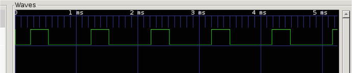
Figure 9-3. pispy capture of 30% PWM signal
That is all there is to using pispy! You can, of course, drag multiple GPIO signals to the display.
One thing you might notice is that the captured.vcd file is usually small in relation to the memory buffers used to capture the data. This is because the file format is used only to record changes in signal. Unless there is significant signal change activity, the VCD file will be smaller.
GTKWave Hints
There are two hints that you should be immediately aware of:
How to get larger height wave forms
How to delete signal traces from the display
Neither one of these are obvious, but in my opinion they should be.
With increasing age, we all eventually suffer from the difficulty of not seeing things up close or things that are too small. According to my optometrist’s office video, it is due to the fact that the lens in our eye can no longer be squeezed by the eye muscles to focus up close. The lens becomes hard and inflexible. Whatever the cause, we can make that wave form a bit more vertically prominent by cheating—by increasing the font size of the Signals window. An increase in font size causes the wave form height to increase with it.
Create a file in your home directory named .gtkwavrc. In it, put the line shown below (modify it to suit your own tastes). The line configures the choice of font and a size for it. The following is what I am using for the examples in this book:
$ cat ~/.gtkwaverc
fontname_signals Monospace 20
At this time, there is no way to delete a trace from the Waves window, but you can achieve the same thing by highlighting the signal to be removed, and then using the Edit menu. Choose Cut and the signal will be removed.
PiSpy in a Nutshell
In this section, I present a bird’s-eye view of how pispy works because it is simply too complex to describe in detail. With this overview, and the provided source code, the keen programmer can reuse the classes found in librpi2 for his or her own programs.
~/pi2/pispy/pispy.cpp
~/pi2/librpi2/*.cpp
~/pi2/include/*.hpp
The pispy command uses the following provided class libraries:
Logic Analyzer (#include "logana.hpp")
GPIO (#include "gpio.hpp")
VCD_Out (#include "vcdout.hpp")
The GPIO class is described in the appendixes. The other classes can be used by the enterprising programmer simply by reviewing the include files for them.
The following basic steps are used by the pispy program to capture and display the signals:
Parse command line options.
Open the kernel mailbox using class LogicAnalyzer’s open() method. This causes the following to happen:
Opens device /dev/rpidma (provided by our rpidma.ko loadable kernel module).
Determines memory allocation offset and flags to use, depending on whether the Raspberry Pi 2 (ARMv7) or prior modules (ARMv6) is being used.
Creates a character device node to access the mailbox with (/dev/logana).
Opens this driver file.
Allocates pages for the mailbox.
Locks that memory.
Obtains a virtual address for the mailbox memory.
GPU memory blocks are allocated for GPIO sampling use (according to option -b).
The first block is accessed where the DMA controller’s first control block will reside (the remainder of each memory block is used for holding samples).
The LogicAnalyzer object’s method propagate() is invoked to clone copies of the first DMA control block to the other memory blocks, making the necessary minor adjustments to chain these together.
If the verbose (-v) option is used, the first control block is displayed on the terminal.
The LogicAnalyzer’s start() method initiates the DMA transfer.
If there are triggers involved, the code waits for the first DMA interrupt to occur. This signals that the data in the first capture block is ready for scanning.
If there are triggers and the trigger condition is found in the first capture block, the capture is allowed to continue until completion.
Otherwise, the current DMA capture is aborted and restarted. The loop will give up if the trigger is not found in so many tries (-T option).
If the verbose option is used (-v), the final DMA status is reported to the terminal session.
At this point the capture is complete and sitting in memory.
The next thing that happens is that the data captured is written out to a file. The capture format used is the *.vcd format (value change dump). This is a format defined by IEEE Standard 1364-1995 in 1995.[1]
The pispy tool then creates or overwrites the file named captured.vcd. It defines signals gpio0 through to gpio31, and writes out timing and change information. This information can then be loaded and viewed directly by the gtkwave command.
After the data is captured in the file, pispy will automatically start the program /usr/bin/gtkwave, unless instructed not to with the option -x. Because gtkwave spits out a lot of GTK messages at startup, these are either suppressed or sent to the file .gtkwave (option -z affects this).
Summary
In this chapter you learned how to apply pispy to capture GPIO signals into a file named captured.vcd, and that this file is normally small compared to the capture memory used. You also learned how to operate gtkwave, which is perhaps less than obvious to use. Finally, the gtkwave customizations provided could be a great help to some.
The next chapter introduces you to the piclk command provided with this book. Using this command, we’ll put the general purpose Raspberry Pi clock to work and use pispy to check our work.
Bibliography
[1] “Value Change Dump”, Wikipedia. http://en.wikipedia.org/wiki/Value_change_dump