2

What Is Federated Learning?

In Chapter 1, Challenges in Big Data and Traditional AI, we examined how shifting tides in big data and machine learning (ML) have set the stage for a novel approach to practical ML applications. This chapter frames federated learning (FL) as the answer to the desire for this new ML approach. In a nutshell, FL is an approach to ML that allows models to be trained in parallel across data sources without the transmission of any data.

The goal of this chapter is to build up the case for the FL approach, with explanations of the necessary conceptual building blocks in order to ensure that you can achieve a similar understanding of the technical aspects and practical usage of FL.

After reading the chapter, you should have a high-level understanding of the FL process and should be able to visualize where the approach slots into real-world problem domains.

In this chapter, we will cover the following topics:

• Understanding the current state of ML
• Distributed learning nature – toward scalable AI
• Understanding FL
• FL system considerations

Understanding the current state of ML

To understand why the benefits derived from the application of FL can outweigh the increased complexity of this approach, it is necessary to understand how ML is currently practiced and the associated limitations. The goal of this section is to provide you with this context.

What is a model?

The term “model” finds usage across numerous different disciplines; however, the generalized definition we are interested in can be narrowed down to a working representation of the dynamics within some desired system. Simply put, we develop a model B of some phenomenon A as a means of better understanding A through the increased interactability offered by B. Consider the phenomenon of an object being dropped from some point in a vacuum. Using kinematic equations, we can compute exactly how long it will take for the object to hit the ground – this is a model of the aforementioned phenomenon.

The power of this approach is the ability to observe results from the created model without having to explicitly interact with the phenomenon in question. For example, the model of the falling object allows us to determine the difference in fall time between a 10 kg object and a 50 kg object at some height without having to physically drop real objects from said height in a real vacuum. Evidently, the modeling of natural phenomena plays a key role in being able to claim a true understanding of said phenomena. Removing the need for the comprehensive observation of a phenomenon allows for true generalization in the decision-making process.

The concept of a model is greatly narrowed down within the context of computer science. In this context, models are algorithms that allow for some key values of a phenomenon to be output given some initial characterization of the phenomenon in question. Going back to the falling object example, a computer science model could entail the computation of values such as the time to hit the ground and the maximum speed given the mass of the object and the height from which it is dropped. These computer science models are uniquely powerful due to the superhuman ability of computers to compute the output from countless starting phenomenon configurations, offering us even greater understanding and generalization.

So, how do we create such models? The first and simplest approach is building rule-based systems or white-box models. A white-box (also known as glass-box or clear-box) model is made by writing down the underlying functions of a system of interest explicitly. This is only possible when information about the system is available a priori. Naturally, in this case, the underlying functions are relatively simple. One such example is the problem of classifying a randomly selected integer as odd or even; we can easily write an algorithm to do this by checking the remainder after dividing the integer by two. If you want to see how much it costs to fill up your gas tank, given how empty the tank is and the price per gallon, you can just multiply those values together. Despite their simplicity, these examples illustrate that simple models can have a lot of practical applications in various fields.

Unfortunately, the white-box modeling of underlying functions can quickly become too complex to perform directly. In general, systems are often too complex for us to be able to construct a white-box model for. For example, let’s say you want to predict the future values of your property. You have a lot of metrics about the property, such as the area, how old it is, its location, and interest rate to name but a few. You believe that there is likely a linear relationship between the property value and all of those metrics, such that the weighted sum of all of them would give you the property value. Now, if you actually try to build a white-box model under that assumption, you will have to directly figure out what the parameter (weight) for each metric is, which implies that you must know the underlying function of the real estate pricing system. Usually, this is not the case. Therefore, we need another approach: black box modeling.

ML – automating the model creation process

The concept of a black box system was first developed in the field of electric circuits during the WWII period. It was the famous cybernetician Norbert Wiener who began treating the black box as an abstract concept, and a general theory was established by Mario Augusto Bunge in the 1960s. The function for estimating future property values, as illustrated earlier, is a good example of a black box. As you might expect, the function is complex enough that it is unreasonable for us to try to write a white-box model to represent it. This is where ML comes in, allowing us to create a model as a black box.

Reference

You might be aware that black box modeling has been criticized for its lack of interpretability, an important concept outside the scope of this book; we recommend Packt’s Interpretable Machine Learning with Python by Serg Masís as a reference on the subject.

ML is a type of artificial intelligence that is used to automatically generate model parameters for making decisions and predictions. Figure 2.1 illustrates this in a very simple way: those cases where the known values and the unknown value have a linear relationship allow a popular algorithm, called ordinary least squares (OLS), to be applied. OLS computes the unknown parameters of the linear relationship by finding the set of parameters that produces the closest predictions on some set of known examples (pairs of input feature value sets and the true output value):

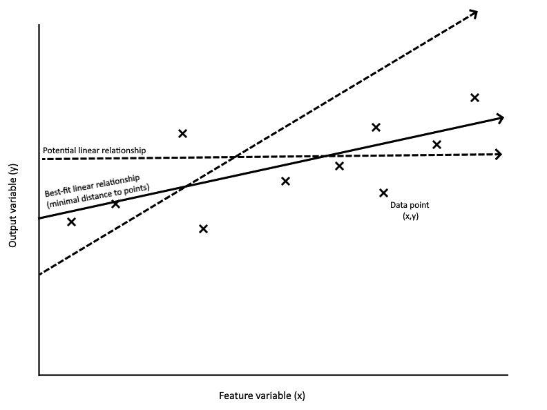
Figure 2.1 – ML determining model parameters

The preceding diagram displays a simple two-dimensional linear regression problem with one feature/input variable and one output variable. In this toy two-dimensional case, it might be relatively straightforward for us to come up with the parameters representing the best-fit relationship directly, either through implicit knowledge or through testing different values. However, it should be clear that this approach quickly becomes intractable as the number of feature variables increases.

OLS allows us to attack this problem from the reverse direction: instead of producing linear relationships and evaluating them on the data, we can use the data to compute the parameters of the best-fit relationship directly instead. Revisiting the real estate problem, let’s assume that we have collected a large number of property valuation data points, consisting of the associated metric values and the sale price. We can apply OLS to take these points and find the relationship between each metric and the sale price for any property (still under the assumption that the true relationship is linear). From this, we can pass in the metric values of our property and get the predicted sale price.

The power of this approach is the abstraction of this relationship computation from any implicit knowledge of the problem. The OLS algorithm doesn’t care what the data represents – it just finds the best line for the data it is given. This class of approaches is exactly what ML entails, granting the power to create models of phenomena without any required knowledge of the internal relationship, given a sufficient amount of data.

In a nutshell, ML lets us program algorithms that can learn to create models from data, and our motivation to do so is to approximate complex systems. It is important to keep in mind that the underlying functions of a complex system can change over time due to outside factors, quickly making models created from old data obsolete. For example, the preceding linear regression model might not work to estimate property values in a far distant future or a faraway district. Variance in such a macroscopic scale is not taken into account in a model containing only a few dozen parameters, and we would need different models for separate groups of adjacent data points – unless we employ even more sophisticated ML approaches such as deep learning.

Deep learning

So, how did deep learning become synonymous with ML in common usage? Deep learning involves the application of a deep neural network (DNN), which is a type of highly-parameterized model inspired by the transmission of signals between neurons in the brain. The foundation of deep learning was established in the early 1960s by Frank Rosenblatt, who is known as the father of deep learning. His work was further developed in the 1970s and 1980s by computer scientists including Geoffrey Hinton, Yann LeCun, and Yoshua Bengio, and the term deep learning was popularized by the University of California, Irvine’s distinguished Professor Rina Dechter. Deep learning can conduct much more complex tasks compared to simpler ML algorithms such as linear regression. While the specifics are beyond the scope of this book, the key problem that deep learning was able to solve was the modeling of complex non-linear relationships, pushing ML as a whole to the forefront of numerous fields due to the increased modeling ability it provided.

This ability has been mathematically proven via specific universal approximation theorems for different model size cases. For those of you who are new to deep learning or ML in general, the third edition of Python Machine Learning by Sebastian Raschka and Vahid Mirjalili is a good reference to learn more about the subject.

Over the past decade, ever-increasingly powerful models have been built by tech giants against the backdrop of big data, as discussed in Chapter 1, Challenges in Big Data and Traditional AI. If we look at the state-of-the-art deep learning models today, they could have up to trillions of parameters; expectedly, this gives them unparalleled flexibility in modeling complex functions. The reason deep learning models can be scaled up to arbitrarily increase performance, unlike other ML model types used previously, is due to a phenomenon called double descent. This refers to the ability for a certain parameterization/training threshold to overcome the standard bias-variance trade-off (where increasing complexity leads to fine-tuning on training data, reducing bias but increasing variance) and continuing to increase performance.

The key takeaway is that the performance of deep learning models can be considered to be limited by just the available compute power and data, two factors that have surged in growth in the past 10 years due to advances in computing and the ever-increasing number of devices and software collecting data, respectively. Deep learning has become intertwined with ML, with deep learning playing a significant role within the current state of ML and big data.

This section focused on establishing a case for the importance of the modeling performed by current ML techniques. In a sense, this can be considered the what – what exactly FL is trying to do. Next, we will focus on the where in terms of the desired setting for numerous ML applications.

Distributed learning nature – toward scalable AI

In this section, we introduce the distributed computing setting and discuss the intersection of this setting with ML approaches to fully establish the support for why FL is necessary. The goal of the section is for the user to understand both the benefits and limitations imposed by the distributed computing setting, in order to understand how FL addresses some of these limitations.

Distributed computing

The past several years have shown a large but predictable rise in the development of new approaches and the conversion of existing server infrastructure within the lens of distributed computing. To generalize further, distributed approaches themselves have shifted more and more from research implementations to extensive use in production settings; one significant example of this phenomenon is the usage of cloud computing platforms such as AWS from Amazon, Google Cloud Platform (GCP) from Google, and Azure from Microsoft. It turns out that the flexibility of on-demand resources allows for cost-saving and efficiency in numerous applications that would, otherwise, be bottlenecked by on-premise servers and computational power.

While a parallel cannot exactly be drawn between cloud computing and the concept of distributed computing, the key benefits stemming from the distributed nature are similar. At a high level, distributed computing involves spreading the work necessary for some computational task over a number of computational agents in a way that allows each to act near-autonomously. The following figure shows the difference between centralized and distributed approaches in the high-level context of answering questions:

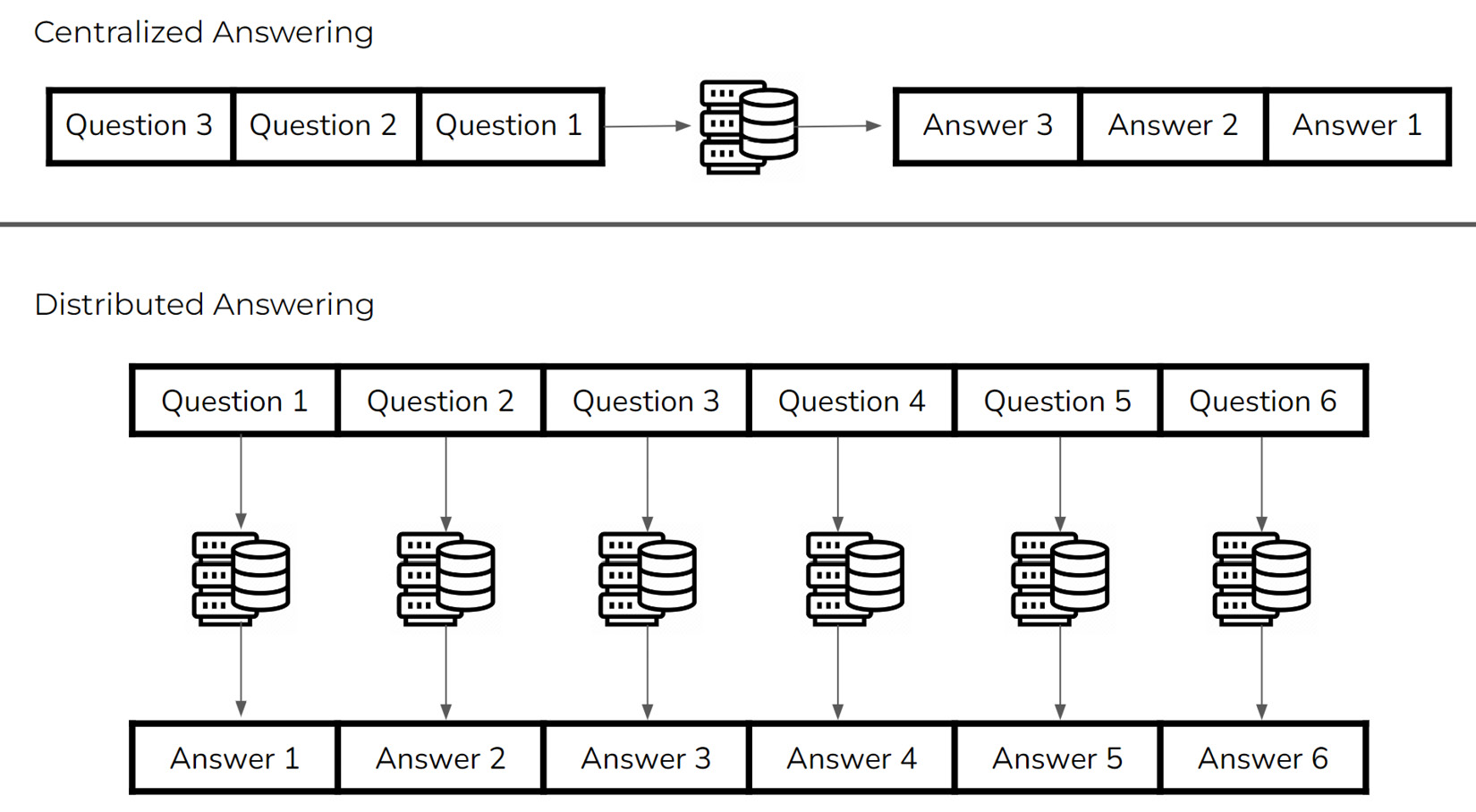
Figure 2.2 – Centralized versus distributed question answering

In this toy example, the centralized approach involves processing the input questions sequentially, whereas the distributed approach is able to process each question at the same time. It should be clear that the parallel approach trades off computational resource usage for increased answering speed. The natural question, then, is whether this trade-off is beneficial for real-world applications.

Real-world example – e-commerce

To understand the practical benefits of distributed computing approaches, let’s analyze an example business problem through a traditional and a distributed computing lens. Consider an e-commerce business that is trying to host its website using on-premise servers. The traditional way to do this would be to perform enough analysis on the business side to determine the expected volume of traffic at some future time and invest in one or a couple of server machines large enough to handle that calculated volume.

Several cases immediately lend themselves to showing the flaws of such an approach. Consider a scenario where usage of the websites greatly exceeds the initial projections. A fixed number of servers means that all upgrades must be hardware upgrades, resulting in old hardware that had to be purchased and is no longer used. Going further, there are no guarantees that the now-increased usage will stay fixed. Further increases in usage will result in more scaling-up costs, while decreases in usage will lead to wasted resources (maintaining large servers when smaller machines would be sufficient). A key point is that the integration of additional servers is non-trivial due to the single-machine approach used to manage hosting. Additionally, we have to consider the hardware limitations of handling large numbers of requests in parallel with one or a few machines. The ability to handle requests in parallel is limited for each machine – significant volumes of traffic would be almost guaranteed to eventually be bottlenecked regardless of the power available to each server.

In comparison, consider the distributed computing-based solution for this problem. Based on the initial business projections, a number of smaller server machines are purchased and each is set up to handle some fixed volume of traffic. If the scenario of incoming traffic exceeding projects arises, no modification to the existing machines is necessary; instead, more similarly-sized servers can be purchased and configured to handle their designated volume of new traffic. If the incoming traffic decreases, the equivalent number of servers can be shut down or shifted to handle other tasks. This means that the same hardware can be used for variable volumes of traffic.

This ability to scale quickly to handle the necessary computational task at any moment is precisely due to how distributed computing approaches allow for computational agents to seamlessly start and stop working on said task. In addition, the use of many smaller machines in parallel, versus using fewer larger machines, means that the number of requests that can be handled at the same time is notably higher. It is clear that a distributed computing approach, in this case, lends itself to cost-saving and flexibility that cannot be matched with more traditional methods.

Benefits of distributed computing

In general, distributed computing approaches offer three main benefits for any computational task – scalability, throughput, and resilience. In the previous case of web hosting, scalability referred to the ability to scale the number of servers deployed based on the amount of incoming traffic, whereas throughput refers to the ability to reduce request processing latency through the inherent parallelism of smaller servers. In this example, resilience could refer to the ability of other deployed servers to take on the load from a server that stops working, allowing the hosting to continue relatively unfazed.

Distributed computing often finds uses when working with large stores of data, especially when attempting to perform analyses on the data using a single machine would be computationally infeasible or otherwise undesirable. In these cases, scalability allows for the deployment of a variable number of agents based on factors such as the desired runtime and amount of data at any given time, whereas the ability of each agent to autonomously work on processing a subset of the data in parallel allows for processing throughput that would be impossible for a single high-power machine to achieve. It turns out that this lack of reliance on cutting-edge hardware leads to further cost savings, as hardware price-to-performance ratios are often not linear.

While the development of parallelized software to operate in a distributed computing setting is non-trivial, hopefully, it is clear that many practical computational tasks greatly benefit from the scalability and throughput achieved by such approaches.

Distributed ML

When thinking about the types of computational tasks that have proven to be valuable in practical applications and that might be directly benefited from increased scalability and throughput, it is clear that the rapidly growing field of ML is near the top. In fact, we can frame ML tasks as a specific example of the aforementioned tasks of analyzing large stores of data, placing emphasis on the data being processed and the nature of the analysis being performed. The joint growth of cheap computational power (for example, smart devices) and the proven benefits of data analysis and modeling have led to companies with both the storage of excessive amounts of data and the desire to extract meaningful insights and predictions from said data.

The second part is exactly what ML is geared to solve, and large amounts of work have already been completed to do so in various domains. However, like other computational tasks, performing ML on large stores of data often leads to a time-computational power trade-off in which more powerful machines are needed to perform such tasks in reasonable amounts of time. As ML algorithms become more computationally and memory-intensive, such as recent state-of-the-art deep learning models with billions of parameters, hardware bottlenecks make increasing the computational power infeasible. As a result, current ML tasks must apply distributed computing approaches to stay cutting-edge while producing results in usable timeframes.

Edge inference

Although the prevalence of deep learning described earlier, besides the paradigm shift from big data to collective intelligence discussed in Chapter 1, Challenges in Big Data and Traditional AI, gives enough motivation for distributed ML, its physical foundation came from the recent development of edge computing. The edge represents the close proximity around deployed solutions; it follows that edge computing refers to processing data at or near the location of the data source. Extending the concept of computation to ML leads to the idea of edge AI, where models are integrated directly into edge devices. A few popular examples would be Amazon Alexa, where edge AI takes care of speech recognition, and self-driving cars that collect real-world data and incrementally improve with edge AI.

The most ubiquitous example is the smartphone – some potential uses are the recommendation of content to the user, searches with voice assistance and auto-complete, auto-sorting of pictures into an album and gallery search, and more. To capitalize on this potential, smartphone manufacturers have already begun integrating ML-focused processor components into the chips they integrate with their newest phones, such as the Neural Processing Unit from Samsung and the Tensor Processing Unit on the Google Tensor chip. Google has also worked to develop ML-focused APIs for Android applications through their Android ML Kit SDK. From this, it should be clear that ML applications are shifting toward the edge computing paradigm.

Let’s say that smartphones need to use a deep learning model for word recommendation. This is so that when you type words on your phone, it gives you suggestions for the next word, with the goal being to save you some time. In the scheme of a centralized computing process, the central server is the only component that has access to this text prediction model and none of the phones have the model stored locally. The central server handles all of the requests sent from the phones to return word recommendations. As you type, your phone has to send what has been typed along with some personal information about you, all the way to the central server. The server receives this information, makes a prediction using the deep learning model, and then sends the result back to the phone. The following figure reflects this scenario:

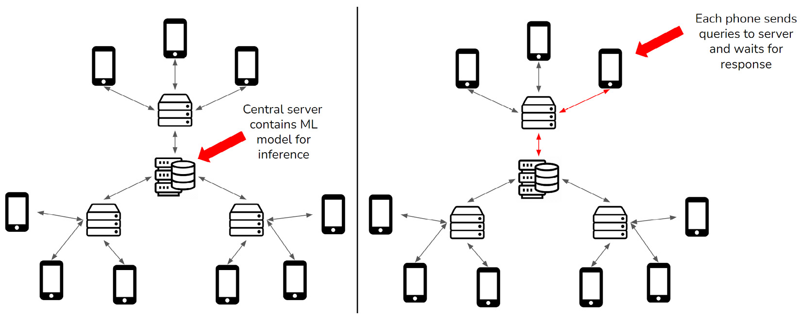
Figure 2.3 – Centralized inference scenario

There are a few problems that become apparent when you look at this scenario. First, even a half to one second of latency makes the recommendation slower than typing everything yourself, making the system useless. Furthermore, if there is no internet connection, the recommendation simply does not work. Another restriction of this scheme is the need for the central server to process all of these requests. Imagine how many smartphones are being used in the world, and you will realize a lack of feasibility due to the extreme scale of this solution.

Now, let’s look at the same problem from the edge computing perspective. What if the smartphones themselves contain the deep learning model? The central server is only in charge of managing the latest trained model and communicating this model with each phone. Now, whenever you start typing, your phone can use the received model locally to make recommendations from what you typed. The following figure reflects this scenario:

Figure 2.4 – Edge inference scenario

This removes both the latency problem and prevents the need to handle the incoming inference requests at a central location. In addition, the phones no longer have to maintain a connection with the server to make a recommendation. Each phone is in charge of fulfilling requests from its user. This is the core benefit of edge computing: we have moved the computing load from the central server to the edge devices/servers.

Edge training

The distinction between centralized and decentralized computing can be extended to the concept of model training. Let’s stick to the smartphone example but think about how we would train the predictive model instead. First, in the centralized ML process, all of the data used to train the recommendation model must be collected from the users’ devices and stored on the central server. Then, the collected data is used to train a model, which is eventually sent to all the phones. This means that the central server still has to be able to handle the large volume of user data coming in and store it in an efficient way to be able to train the model.

This design leads to the problems found in the centralized computing approach: as the number of phones connected to the server increases, the server’s ability to work with the incoming data needs to scale in order to maintain the training process. In addition, since the data needs to be transmitted and stored centrally in this approach, there is always the possibility of the interception of transmissions or even attacks on the stored data. There are several cases where data confidentiality and privacy are required or strongly desired; for example, applications in the financial and medical industries. Centralized model training thus limits use cases, and an alternative way to work with data directly on edge devices is required. This exact setting is the motivation for FL.

Understanding FL

This section focuses on providing a high-level technical understanding of how FL actually slots in as a solution to the problem setting described in the previous section. The goal of this section is for you to understand how FL fits as a solution, and to provide a conceptual basis that will be filled in by the subsequent chapters.

Defining FL

Federated learning is a method to synthesize global models from local models trained on the edge. FL was first developed by Google in 2016 for their Gboard application, which incorporates the context of an Android user’s typing history to suggest corrections and propose candidates for subsequent words. Indeed, this is the exact word recommendation problem discussed in the Edge inference and Edge training sections. The solution that Google produced was a decentralized training approach where an iterative process would compute model training updates at the edge, aggregating these updates to produce the global update to be applied to the model. This core concept of aggregating model updates was key in allowing for a single, performant model to be produced from edge training.

Let’s break this concept down further. The desired model is distributed across the edge and is trained on data collected locally at the edge. Of course, we can expect that a model trained on one specific data source is not going to be representative of the entire dataset. As a result, we dub such models trained with limited data local models. One immediate benefit of this approach is the enabling of ML on data that would otherwise not be collected in the centralized case, due to issues with privacy and efficiency.

Aggregation, the key theoretical step of FL, allows for our desired single global model to be created from the set of local models produced at some iteration. The most well-known aggregation algorithm, popular for its simplicity and surprising performance, is called federated averaging (FedAvg). FedAvg is performed on a set of local models by computing the parameter-wise arithmetic mean across the models, producing an aggregate model. It is important to understand that performing aggregation once is not enough to produce a good global aggregate model; instead, it is the iterative process of locally training the previous global model and aggregating the produced local models into a new global model that allows for global training progress to be made.

The FL process

To better understand FL from an iterative process perspective, we break it down into the core constituent steps of a single iteration, or round.

The steps for a round can be described as follows:

1. The aggregate global model parameters are sent to each user’s device.
2. The received ML models located on the user devices are trained with local data.
3. After a certain amount of training, the local model parameters are sent to the central server.
4. The central server aggregates the local models by applying an aggregation function, producing a new aggregate global model.

These steps are depicted in Figure 2.5:

Figure 2.5 – FL steps

The flow from steps 1 to 4 constitutes a single round of FL. The next round begins as the user servers/devices receive the newly created aggregate model and start training on the local data.

Let’s revisit Google’s word recommendation for Gboard. At some point in time, each phone stores a sufficient amount of its user’s typing data. The edge training process can create a local model from it, and the parameters will be sent to the central server. After receiving parameters from a certain number of phones, the server aggregates them to create a global model and sends it to the phones. This way, every phone connected to the server receives a model that reflects local data in all of the phones without ever transmitting the data from them. In turn, each phone retrains the model when another batch of sufficient data is collected, sends the model to the server, and receives a new global model. This cycle repeats itself over and over according to the configuration of the FL system, resulting in the continuous monitoring and updating of the global model.

Note that the user data never leaves the edge, only the model parameters; nor is there a need to put all the data in a central server to generate a global model, allowing for data minimalism. Moreover, model bias can be mitigated with FL methods, as discussed in Chapter 3, Workings of the Federated Learning System. That is why FL can be regarded as a solution to the three issues of big data, which were introduced in Chapter 1, Challenges in Big Data and Traditional AI.

Transfer learning

FL is closely related to an ML concept called transfer learning (TL). TL allows us to use large deep learning models that have been trained by researchers using plentiful compute power and resources on very generalized datasets. These models can be applied to more specific problems.

For example, we can take an object detection model trained to locate and name specific objects in images and retrain it on a limited dataset containing specific objects we are interested in, which were not included in the original data. If you were to take the original data, add to it the data of those objects of our interest, and then train a model from scratch, a lot of computational time and power would be required. With TL, you can quicken the process by leveraging a key fact about those existing large, generalized models. There is a tendency for the intermediate layers of large DNNs to be excellent at extracting features, used by the following layers for the specific ML task. We can maintain its learned ability to extract features by preserving the parameters in those layers.

In other words, parameters in certain layers of existing pre-trained models can be preserved and used to detect new objects – we do not need to reinvent the wheel. This technique is called parameter freezing. In FL, model training often takes place in local devices/servers with limited computational power. One example using the Gboard scenario is performing parameter freezing on a pretrained word embedding layer to allow training to focus on task-specific information, leveraging prior training of the embeddings to greatly reduce the trainable parameter count.

Taking this concept further, the intersection of FL and TL is called federated transfer learning (FTL). FTL allows for the FL approach to be applied in cases where the local datasets differ in structure by performing FL on a shared subset of the model that can later be extended for specific tasks. For example, a sentiment analysis model and a text summarization model could both share a sentence encoding component, which can be trained using FL and used for both tasks. TL (and, by extension, FTL) are key concepts that allow for training efficiency and incremental improvement to be realized in FL.

Personalization

When edge devices are dealing with data that is not independent and identically distributed (IID), each device can customize the global model. This is an idea called personalization, which can be considered as fine-tuning the global model with local data, or the strategic use of bias in the data.

For example, consider a shopping mall chain that operates in two areas with distinct local demographics (that is, the chain deals with non-IID data). If the chain seeks tenant recommendations for both locations using FL, each of the locations can be better served with personalized models than a single global model, helping attract local customers. Since the personalized model is fine-tuned or biased with local data, we can expect that its performance on general data would not be as good as that of the global model. On the other hand, we can also expect that the personalized model performs better than the global model on the local data for which the model is personalized. There is a trade-off between user-specific performance and generalizability, and the power of an FL system comes from its flexibility to balance them according to the requirements.

Horizontal and vertical FL

There are two types of FL: horizontal or homogeneous FL and vertical or heterogeneous FL. Horizontal FL, also called sample-based FL, is applicable when all local datasets connected with the aggregator server have the same features but contain different samples. The Gboard application discussed earlier is a good example of horizontal FL in the form of cross-device FL, that is, local training taking place in edge devices. The datasets in all Android phones have identical formats but unique contents that reflect their user’s typing history. On the other hand, vertical FL, or feature-based FL, is a more advanced technology that allows parties holding different features for the same samples to cooperatively generate a global model.

For example, a bank and an e-commerce company might both store the data of residents in a city but their features would differ: the former knows the credit and expenditure patterns of the citizens, the latter their shopping behavior. Both of them can benefit by sharing valuable insights without sharing customer data. First, the bank and e-commerce company can identify their common users with a technique called private set intersection (PSI) while preserving data privacy using Rivest-Shamir-Adleman (RSA) encryption. Next, each party trains a preliminary model with local data containing unique features. Those models are then aggregated to construct a global model. Usually, vertical FL involves multiple data silos, and when that is the case, it is also called cross-silo FL. In China, federated Ai ecosystem (FATE) is well known for its seminal demonstration of vertical FL involving WeBank. If you are interested in further conceptual details of FL, there is a very illustrative and well-written report by Cloudera Fast Forward Labs, at https://federated.fastforwardlabs.com/.

The information on FL contained in this section should be sufficient to understand the following chapters, which examine, in further depth, some of the key concepts introduced here. The final section of the chapter aims to cover some of the auxiliary concepts focused on the practical application of FL.

FL system considerations

This section mainly focuses on the multi-party computation aspects of FL, including theoretical security measures and full decentralization approaches. The goal of this section is for you to be aware of some of the more practical considerations that should be taken into account for practical FL applications.

Security for FL systems

Despite the nascency of the technology, experimental usage of FL has emerged in a few sectors. Specifically, anti-money laundering (AML) in the financial industry and drug discovery and diagnosis in the medical industry have seen promising results, as proofs of concepts in those fields have been successfully conducted by companies such as Consilient and Owkin. In AML use cases, banks can cooperate with one another to identify fraudulent transactions efficiently without sharing their account data; and hospitals can keep their patient data to themselves while improving ML models for detecting health issues.

These solutions exploit the power of relatively simple horizontal cross-silo FL, as explained in the Understanding FL section, and its application is spreading to other areas. For example, Edgify is a UK-based company contributing to the automation of cashiers at retail stores in collaboration with Intel and Hewlett Packard. In Munich, Germany, another UK-based company, Fetch.ai, is developing a smart city infrastructure with their FL-based technology. It is clear that the practical application of FL is rapidly growing.

Although FL can circumvent the concern over data privacy thanks to its privacy-by-design (model parameters do not expose privacy) and data minimalist (data is not collected in the central server) approach, as discussed in Chapter 1, Challenges in Big Data and Traditional AI, there are potential obstructions against its implementation; one such example is mistrust among the participants of an FL project. Consider a situation where Bank A and Bank B agree to use FL for developing a collaborative AML solution. They decide on the common model architecture so that each can train a local model with their own data and aggregate the results to create a global model to be used by both.

Naïve implementations of FL might allow for one bank to reconstruct the local model from the other bank, using their local model and the aggregate model. From this, the bank might be able to extract key information on the data used to train the other bank’s model. As a result, there might be a dispute regarding which party should host the server to aggregate the local models. A possible solution is having a third party host the server and take responsibility for model aggregation. Yet, how would Bank A know that the third party is not colluding with Bank B, and vice versa? Going further, the integration of an FL system into a security-focused domain leads to new concerns regarding the security and stability of each system component. Known security issues tied to different FL system approaches might incur an additional potential weakness to adversarial attacks that outweighs the benefits of the approach.

There are several security measures to allow FL collaboration without forcing the participants to trust one another. With a statistical method called differential privacy (DP), each participant can add random noise to their local model parameters to prevent the ability to glean information on the training data distribution or specific elements from the transmitted parameters. By sampling the random noise from a symmetric distribution with zero mean and relatively low variance (for example, Gaussian, Laplace), the random differences added to the local models are expected to cancel out when aggregation is performed. As a result, the global model is expected to be very similar to what would have been generated without DP.

However, there is a critical limitation to this approach; for the sum of the added random noise to converge to zero, a sufficient number of parties must participate in the coalition. This might not be the case for projects involving only a few banks or hospitals, and using DP in such cases would harm the global model’s integrity. Some additional measures would be necessary, for example, each participant sending multiple copies of their local model to increase the number of models so that the noise will be offset. Another possibility in certain fully-decentralized FL systems is secure multi-party computation (MPC). MPC-based aggregation allows agents to communicate among themselves and compute the aggregate model without involving a trusted third-party server, maintaining model parameter privacy.

How could the participants secure the system from outside attacks? Homomorphic encryption (HE), which preserves the effects of addition and multiplication on data across encryption, allows the local models to be aggregated into the global model in an encrypted form. This precludes the exposure of model parameters to outsiders who do not possess the key for decryption. Yet, HE’s effectiveness in securing the communication between the participants comes with a prohibitively high computational cost: processing the operation on data with the HE algorithm can take hundreds of trillions of times longer than otherwise!

A solution to mitigate this challenge is the use of partial HE, which is compatible with only one of the additive or multiplicative operations across encryption; therefore it is computationally much lighter than the fully homomorphic counterpart. Using this scheme, each participant in a coalition can encrypt and send their local model to the aggregator, which then sums up all local models and sends the aggregated model back to the participants, who, in turn, decrypt the model and divide its parameters by the number of participants to receive the global model.

Both HE and DP are essential technology for the practical application of FL. Those interested in the implementation of FL in real-world scenarios can learn a great deal from Federated AI for Real-World Business Scenarios written by IBM Research Fellow Dinesh C. Verma.

Decentralized FL and blockchain

The architecture of FL discussed so far is based on client-server networks, that is, edge devices exchanging models with a central aggregator server. Due to the issues surrounding trust between the participants of FL coalitions discussed earlier; however, building a system with an aggregator as a separate and central entity can be problematic. It can be difficult for the host of an aggregator to be impartial and unbiased toward their own data. Also, having a central server inevitably leads to a single point of failure in the FL system, which results in low resilience. Furthermore, if the aggregator is set up in a cloud server, the implementation of such an FL system would require a skilled DevOps engineer, who might be difficult to find and expensive to hire.

Given these concerns, Kiyoshi Nakayama (the primary author of this book) co-authored an article about the first-ever experimentation of a fully decentralized FL system using blockchain technology (http://www.kiyoshi-nakayama.com/publications/BAFFLE.pdf). Leveraging smart contracts to coordinate model updates and aggregation, a private Ethereum network was constructed to perform FL in a serverless manner. The results of the experiment showed that a peer-to-peer, decentralized FL can be much more efficient and scalable than an aggregator-based, centralized FL. The superiority of decentralized architecture was confirmed in a more recent experiment conducted by Hewlett Packard and German research institutes who gave a unique name to decentralized FL with blockchain technology: swarm learning.

While research and development in the field of FL are shifting to a decentralized model, the rest of this book assumes centralized architecture with an aggregator server. There are two reasons for this design. First, blockchain is still a nascent technology that AI and ML researchers are not necessarily familiar with. Incorporating a peer-to-peer communication scheme can overcomplicate the subject matter. And second, the logic of FL itself is independent of the network architecture, and there is no problem with the centralized model to illustrate how FL works.

Summary

In this chapter, we covered the two key developments that have resulted from the recent growth in accessible computational power at all levels. First, we looked at the importance of models and how this has enabled ML to grow considerably in practical usage, with increases in computational power allowing stronger models that surpass manually created white-box systems to continuously be produced. We called this the what of FL – ML is what we are trying to perform using FL.

Then, we took a step back to look at how edge devices are reaching a stage where complex computations can be performed within reasonable timeframes for real-world applications, such as the text recommendation models on our phones. We called this the where of FL – the setting where we want to perform ML.

From the what and the where, we get the intersection of these two developments – the usage of ML models directly on edge devices. Remember that the standard central training approach for ML models greatly suffers from the need to centrally collect all of the data in the edge ML case, as this prevents applications requiring efficient communication or data privacy from being possible. We showed that FL directly addresses this problem by performing all training at the edge to produce local models, at the same location as the requisite data stores. Aggregation algorithms take these local models and produce a global model. By iteratively switching between local training and aggregation, FL allows for the creation of a model that has effectively been trained across all data stores without ever needing to centrally collect the data.

We concluded the chapter by stepping outside the theory behind effective aggregation, looking at system and architecture design considerations regarding aspects such as model privacy and full decentralization. After reading the chapter, it should be clear that the current state of ML, edge computing, and fledgling growth in practical FL applications makes it clear that FL is poised for serious growth in the near future.

In the next chapter, we will examine the implementation of FL from a system-level perspective.

Further reading

To learn more about the topics that were covered in this chapter, please take a look at the following references:

• Ruiz, N. W. (2020, December 22). The Future is Federated. Medium.
• Contessa, G. (2010). Scientific Models and Fictional Objects. Synthese, 172(2): 215–229.
• Frigg, R. and Hartmann, S. (2020). Models in Science. In Zalta, E. N. (ed.). The Stanford Encyclopedia of Philosophy.
• Bunge, M. (1963). A General Black Box Theory. Philosophy of Science, 30(4): 346-358.
• Moore, S. K., Schneider, D. and Strickland, E. (2021, September 28). How Deep Learning Works: Inside the neural networks that power today’s AI. IEEE Spectrum.
• Raschka, S. and Mirjalili, V. (2019). Python Machine Learning: Machine Learning and Deep Learning with Python, scikit-learn, and TensorFlow 2 (3rd Ed.). Birmingham: Packt Publishing.
• McMahan, B., Moore, E., Ramage, D., Hampson, S., and y Arcas, B. A. (2016). Communication-efficient learning of deep networks from decentralized data. JMLR WandCP, 54.
• Huang, X., Ding, Y., Jiang, Z. L. and Qi, S. (2020). DP-FL: a novel differentially private federated learning framework for the unbalanced data. World Wide Web, 23: 2529–254.
• Yang, Q., Liu, Y., Chen, T., and Tong, Y. (2019). Federated Machine Learning: Concept and Applications. ACM Transactions on Intelligent Systems and Technology (TIST), 10(2), 1-19.
• Verma, D. C. (2021). Federated AI for Real-World Business Scenarios. Florida: CRC Press.
• Ramanan, P., and Nakayama, K. (2020). Baffle: Blockchain Based Aggregator Free Federated Learning. 2020 IEEE International Conference on Blockchain, 72-81.
• Warnat-Herresthal, S., Schultze, H., Shastry, K. L., Manamohan, S., Mukherjee, S., Garg, V., and Schultze, J. L. (2021). Swarm Learning for decentralized and confidential clinical machine learning. Nature, 594(7862), 265-270.