
3
Futures Contracts and Forward Contracts
A futures contract is a commitment to buy or sell an underlying asset at a certain price, at a future date. The term “underlying asset” is used in a generic sense: contracts may involve both commodities as well as financial securities, or again, other underlying assets such as temperatures or precipitation (in the case of climatic derivatives). Any commitment to sell (or buy) involves, on the part of a counterparty, a reciprocal and irrevocable commitment to buy (or to sell). Futures markets are organized markets, where futures contracts are negotiated. Forward contracts are contracts concluded over the counter (OTC), which reciprocally engage a buyer and a seller to carry out a physical operation at a later date. The price, the quality and the quantities are fixed at the time that the contract is drawn up.
Futures and forwards share certain similarities but differ on essential points. In both cases, there is a commitment for execution at a later date. However, three differences must be highlighted:
- – futures are contracts where a clearing house (CH) serves as an intermediary and guarantee between contracting parties, while forwards are over the counter contracts;
- – apart from exceptional cases, forwards end in a physical delivery, while the majority of futures do not lead to a delivery of the underlying asset;
- – the temporal flow profiles are different for both instruments.
It must also be highlighted that futures contracts are generally much more liquid than forward contracts, although there do exist certain notable exceptions to this rule1.
3.1. Futures markets in 2013 and 2014
Stock exchanges are private enterprises that engage in keen competition. This competition translates into mergers and acquisitions, and also demergers (for example, a part of Euronext quit the ICE group in 2014). This competition is also reflected in a constantly changing range of products that are offered to investors. Stock exchanges share a lot of information about their activity and we recommended that the reader visit their official websites. The characteristics of contracts, market statistics, live or slightly delayed listings, order books, etc. are generally available here.
Table 3.1 shows the growth of future markets.
Table 3.1. The hierarchy of organized markets in 2013 and 2014 (in millions of contracts) [CYC 15]
| The major future markets around the world in 2013 and 2014 | ||
| 2013 | 2014 | |
| CME Group | 3,160 | 3,443 |
| Shanghai | 1,285 | 1,685 |
| Dalian | 1,401 | 1,539 |
| Eurex | 1,554 | 1,492 |
| Zhengzhou | 1,051 | 1,353 |
| ICE Group | 663 | 707 |
| Osaka | 265 | 253 |
| Euronext Paris | n-a | 1 44 |
OBSERVATION REGARDING TABLE 3.1.– CME, Chicago Mercantile Exchange (United States of America); ICE, Intercontinental Exchange (United States of America); Eurex is a joint subsidiary of the Frankfurt and Zurich stock exchanges; Dalian, Shanghai and Zhengzou are fast-growing Chinese stock exchanges.
In a very short span of time, Asian markets have established themselves in a prominent position, as can be seen in Table 3.2. This change reflects the continuous increase in and growing sophistication of commodity trading in China.
3.2. Derivative markets in 2016
Table 3.2. The rise in power of the Chinese organized markets2

3.3. An overview of futures contracts
3.3.1. Notations
Unless otherwise specified, 0 designates the point at which a transaction is initiated, T designates the maturity date of the futures contract under consideration and t designates a point in the future that precedes the maturity date: 0 < t < T. However, it must be noted that if 0 designates the point at which an initial position is taken by an agent, it moves over the course of time. In other cases, 0 designates the point at which we may begin negotiating a contract. In each case, the notations must be specified.
There is no stable set of notations in academic literature, nor in professional literature, and hence the reader must pay attention to context.
A futures contract links a buyer and a seller. The buyer has made the irrevocable commitment to buy, on the date T, an asset that is said to be the underlying entity of the contract. The seller has made the irrevocable commitment to deliver, on the date T, the underlying asset. The price that the buyer pays and at which the seller delivers the asset, at the time T, is fixed when the contract is drawn up at the time 0, predating T. Consequently, 0 then denotes the point in time at which the contract was drawn up. F0,T designates the prices, stipulated on the date 0, for the delivery of the support on the date of maturity, T. More generally, Ft,T designates the futures price prevailing at the time t, for t ϵ [0,T] . For t ϵ [0,T], Ct represents the spot price of the underlying asset. We use “spot price”, “physical price” or “cash price”. In a very general manner, Ft,T ≠ Ct. The basis is thus defined as: Bt,T ≡ Ft,T − Ct. Apart from a few exceptions, arbitrage operations lead the market to a situation at maturity such that FT,T = CT ⇔ BT,T = 0.
More generally, the basis Bt,T normally tends to zero when t tends toward T, as illustrated in the following graph: the explanation for the change resulting from arbitrage operations will be given later on in the text.
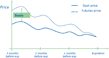
Figure 3.1. The basis narrows and then cancels itself out as maturity approaches
(source: Euronext)
3.3.2. Gains and losses at the maturity of an elementary operation
The vocabulary that is ordinarily used to talk about futures markets may be misleading: at the date 0, the buyer buys nothing and only commits to buying a certain quantity of some entity on the date T and at the price F0,T. In the same way, the seller sells nothing at the time 0. They only commit to selling a certain quantity of a certain underlying asset on the date T, at the price F0,T. To avoid ambiguity, we should specify “the operator who has committed to sell” and “the operator who has committed to buy”. However, for convenience’s sake we use the terms “seller” and “buyer”. Readers who approach future markets will be advised to keep this in mind.
3.3.2.1. Financial results of an operation that was initiated at t = 0 and that terminated at t = T
At the time of maturity, T, the financial results of the operation that the buyer committed to on the future market at the time 0, can be expressed as: (FT,T − F0,T). If the price of the underlying entity has increased between 0 and T, then the buyer has realized a gain; in case the price has dropped between 0 and T, the buyer suffers a loss. The seller’s result at the time of maturity is equal to (F0,T − FT,T). If the price of the underlying entity has increased, between 0 and T, then the seller suffers a loss; if the prices have dropped between 0 and T, then the seller realizes a gain. An important point: what one party gains the other loses. Thus, overall, operations on futures markets make up a zero-sum game. In other words, a global speculator can expect zero gains on the futures market. More precisely, they may even have a slightly negative gain as operators must pay commissions to the CH, pay intermediaries and pay taxes.
3.3.2.2. The temporal profile of financial flows resulting from a futures contract between t = 0 and t = T
In the case of a futures contract, initiated at t = 0 and terminating at t = T, the overall margin (FT,T − F0,T) is paid in the form of successive flows at the closing of the markets every day. In practice, the CH computes the daily change in position. For example, between the date (t − 1) and the date t, the financial flow resulting from a contract is equal to |Ft,T − F(t − 1),T|. If Ft,T > F(t − 1),T, this flow is positive for the buyer and negative for the seller; conversely, if Ft,T < F(t − 1),T, the flow is negative for the buyer and positive for the seller. This series of flows resulting from the futures contract for the operator in the buyer’s position is indicated in Table 3.3, assuming that the operator conserves their position until the date of maturity T :
Table 3.3. Daily gains or losses for the operator in the buyer’s position in a futures contract [PON 96]
| Day | 0 | 1 | t | T | Total |
| Flux | 0 | F1,T − F0,T | Ft,T − F(t − 1),T | FT,T − F(T − 1),T | FT,T − F0,T |
We can easily verify that 0 + (F1,T − F0,T) + … + (Ft,T − F(t − 1),T) + … + (FT,T − F(T − 1),T) = FT,T − F0,T.. The flows generated for the operator in the seller’s position are simply the opposite of the flows generated for the operator in the buyer’s position.
NOTE.– The initial flow of a futures contract is not strictly zero, as the operators pay the CH a commission when they take a position. However, this commission is small enough to be considered negligible in this overview of fundamental principles. Table 3.3 also does not take into account the deposit that is paid on the first day, as this deposit is refunded at the date of maturity. Further, the freezing of capital represents a cost but this is low enough to not be taken into account.
The flows paid or received daily are margin calls, payable or receivable, depending on the case. After the markets close for the day, the CH credits or debits the corresponding sums to/from the operators’ accounts; consequently, the operators who suffer a negative flow on the evening of the day t must immediately deposit funds into their account. This constraint weighs quite heavily on operators who must ensure on a daily basis that they have enough liquid funds to cover the margin calls.
Depending on the changes in the price of the underlying asset, every operator will realize a loss or gain every day. The financial result of the position that began at t = 0 and closed on t = T is, quite simply, equal to the sum of the payable and receivable margin calls resulting from the position. More generally, the financial result of any position taken is equal to the sum of the daily flows generated between the time that this position is taken up and the time that it is given up.
3.3.2.3. Officials on the future market take very few financial risks
The following point is very important in order to understand the functioning of futures markets: every day, the fluctuations in the price of the underlying asset lead to certain operators suffering losses and other realizing gains. Let us recall that we speak here of daily gains or losses. An operator may very well realize an overall profit, taken across the period from which they took up the position to the time it ended, while suffering a loss in the course of 1 day. In this case, the loss over 1 day will only diminish the overall gain accumulated from the time the initial position was taken.
Losses and gains only become fully effective when operators retire from the market, either at the time of maturity, T, or before the date of maturity. While waiting for operators to leave the market, the CH credits potential gains in the form of payable margin calls to the account of the operator who is virtually winning. As long as the operator who emerges ahead remains on the market – that is, as long as they keep their position open – they cannot use the liquidities paid into their account from the CH.
In order to credit daily gains into the accounts of the winning operators, the CH imposes payable margin calls on those who have realized losses in the day (the losers). The financial risk taken by the CH is, therefore, very small, as it only involves payable margin calls that certain losers may not be able to cover. In cases where this may occur:
- – the CH can liquidate the guarantee deposit that the operator (who is unable to pay their margin call) has made at the time they took up their position;
- – in the case that this is not enough, the CH has its own funds that allow it to cover any eventual losses;
- – the CH also has insurance in place.
However, these situations are exceptional, as, a priori, only operators with solid financial guarantees are allowed to enter the futures markets. If an operator is unable to pay their margin calls, they incur a loss and are then excluded from the market, i.e. their position is closed by the CH.
3.3.3. Closing a position before maturity
Let us take the example of a long position – that is the buyer’s position – for a contract that came into effect on the date 0 in the past; at the end of the day t, the operator sells a contract whose date of maturity is T at the price Ft,T. This is the same as closing their position, as the operator is simultaneously the buyer and seller for the same date of maturity T. The financial results following this closing of the position are presented in Table 3.4.
Table 3.4. Daily gains or losses resulting from a position being closed [PON 96]
| t | t +1 | T | |
| Contract bought at time 0 Contract sold on date t Total net |
Ft,T − F(t − 1),T Ft,T − Ft,T = 0 Ft − F(t − 1) |
F(t+1),T − Ft,T Ft,T − F(t+1),T 0 |
FT,T − F(T − 1),T F(T − 1),T − FT,T 0 |
This table emphasizes that the position taken from the day t systematically generates two opposite flows, hence a zero sum, which is normal as the operator is simultaneously in the position of the buyer and the seller for the same support, the same price and the same date of maturity. It is then said that the initial long position has been cancelled or closed as the new position – which adds purchase and selling to the same contract – only generates null flows over the interval [t + 1; T]. The initial position taken, preserved over the interval [0; t], has thus produced a result equal to (Ft,T − F0,T), then 0 + (F1,T − F0,T)+ (F2,T − F1,T)+ … + (F(t − 1),T − F(t − 2),T)+ (Ft,T − F(t − 1),T) = Ft,T − F0,T.
This table clearly shows one of the key advantages of futures markets: at the time t, earlier than T, any player may liquidate the gains or losses resulting from the position taken earlier at the time t = 0. However, it must be noted that in order to make full use of this advantage, it is essential that the futures market be sufficiently liquid.
3.4. Arbitrage operations and conditions for no arbitrage
“A pure arbitrage is an operation that excludes all risk of a negative flow but involves the possibility of a positive flow with a non-null probability” [PON 96]. The no arbitrage (NA) hypothesis plays a central role in economics and financial mathematics; it is intrinsically linked to the concept of a complete market. A market is intuitively considered as being complete if any new asset can be created from existing assets, which signifies that there is no purpose in inventing new instruments ex nihilo, as they can be synthesized from existing elements; the concept of a complete market is difficult to approach formally. However, we will provide a brief outline of the concept as it is indispensable for an understanding of the pricing of financial instruments.
An opportunity for arbitrage arises notably when it is possible to replicate the flows resulting from an asset by creating a portfolio made up of m other assets. To be more precise, an arbitrage opportunity emerges when a portfolio that replicates an asset may be created at a price different from the market price of the replicated asset. We say that a portfolio – made up of a collection of assets – replicates, duplicates or synthesizes another existing asset if it produces the same flows as this asset. It can be easily understood that if the price of the portfolio and the price of the duplicated asset are not identical, then an opportunity for arbitrage emerges. For example, if the duplication portfolio is less costly than the duplicated asset, it is enough to sell the asset and to buy the portfolio. We then have a strictly positive initial flow when we begin such an arbitrage. It is important to understand that selling an asset is the same as committing to pay a series of financial flows; the portfolio will then result in a series of flows that the arbitrageur will transfer to the buyer of the replicated asset. The sum of the arbitrageur’s inflows and outflows thus becomes zero in each period, but as the abritrageur obtained a strictly positive initial flow the operation is profitable.
3.4.1. An elementary example of arbitrage through replication [BOS 02]
Three assets A, B and C are traded on a financial market. If A is purchased on the date 0, a flow F1 is generated on the date t = 1 and a flow F2 is generated on t = 2; if A is sold, these two flows must be paid; the holder of a financial asset B will receive a flow on t = 1 and the holder of C will receive a flow on t = 2. Table 3.5 gives the characteristics of these three assets; P0 designates the price on the date t = 0:
Table 3.5. Arbitrage opportunity [BOS 02]
| P0 | F1 | F2 | |
| A | 1,000 $ | 100 $ | 1,100 $ |
| B | 95 $ | 100 $ | 0 $ |
| C | 80 $ | 0 $ | 100 $ |
- a) the portfolio PA = {1B ; 11C} replicates the flows resulting from A, as the holder of PA receives 100 $ on t = 1 and 1,100 $ on t = 2, i.e. exactly what a holder of A would receive;
- b) the price of PA is 95 + (11 × 80) = 975 $. The price of PA is lower than that of A, while both these assets have the same flows; an arbitrageur would make use of this opportunity by buying PA, the underestimated asset and by selling A, the overestimated asset.
The initial flow F0 generated by this arbitrage is equal to 25 $; consequently, the portfolio PA generates a flow F1 = 100 $, and then a flow F2 = 1, 100 $, which is refunded to the holder of the asset A, which the arbitrageur has sold.
The series of flows for the arbitrageur is, therefore, {+25 $; 0 $; 0 $}; the opportunity for arbitrage is evident. It is in the arbitrageur’s interest to multiply this operation and they will, thus:
- – massively buy the portfolio PA (that is the assets B and C);
- – massively sell the title A.
Having done this, the arbitrageur will then cause an increase in the prices of B and C and a reduction in the price of A; at a certain point, the arbitrage opportunity will disappear. This is a peculiarity of arbitrage operations: acting on arbitrage opportunities leads to the re-establishment of an NA situation.
3.4.2. A formal definition of NA [PON 96]
Let us consider an asset A, which will result in the flows FA(t), in the future (t > 0) ; these flows may be determinist or random. A portfolio composed of m assets is characterized by an m-tuple (n1, … nk, … nm), where nk designates the number of assets k that make up the portfolio:
- – if nk > 0, the asset k is held in the portfolio and results in inflows;
- – if nk < 0, the holder of the portfolio is in the position of a seller for this asset (they hold the short position), which leads to outflows.
The portfolio PA, characterized by the m-tuple (n1, …, nm), duplicates the asset A if:

We can also say that the portfolio PA synthesizes or replicates the asset A. π(k) denotes the price of the asset k. When PA = (n1, … nk, … nm) replicates the asset A, the absence of an opportunity for arbitrage (NA) is translated by the equality between the price of any asset A and the price of any replication portfolio PA:

where π(PA) is the price of the portfolio PA and π(A) is the price of the asset A.
3.5. Hedging operations
The aim of any hedging operation is to reduce – or eventually cancel out – the price risk associated with a preexisting position. For example, a trader who holds a stock of commodities that must be preserved until a date τ is subject to the risk of prices dropping. The need for hedging emerges when an operator is obliged to retain a risky position. In the above example, we can easily imagine a trader who must preserve their stock until the date τ in order to be certain of having it when the delivery is needed.
A hedging operation consists of taking a new position that is characterized by a risk that is negatively correlated with the preexisting risk. Taking the above example of a trader holding a stock of commodities, the fundamental principle here consists of taking a position that will result in a gain if the price of the commodity drops around the time τ. If the trader uses futures contracts, they must take the position of the seller as this would result in gains in case of a drop in the price of the support. The trader’s hedging strategy would thus consist of:
- – maintaining their long position, that is preserving their stock of commodities;
- – taking a short position on a futures market.
The combination of these two positions defines a hedging operation or hedge. This reduces the financial risk that characterizes the initial position as the eventual diminished value of the stock will, at least partially, be compensated by a financial gain on the futures market. On the other hand, if the price of the commodity increases, the rise in the value of the stock on the physical market will be accompanied by a loss on the futures market (a financial market).
Hedging may be total (rare) or partial (most frequent). When a hedger uses futures contracts, they choose derivative contracts based on an underlying support that is as close as possible to the preexisting asset. When the underlying support is identical to the asset to be hedged, the hedge may be perfect.
3.5.1. An elementary example of hedging
Let us take the example of a milling wheat producer: between the time of sowing, in spring in the year N, and the time of sale, December, this agricultural producer based in Brie is subject to the risk of a drop in prices. There exists a futures market for milling wheat on Euronext Paris: a possible hedge that is very easy to implement consists of the agricultural producer committing to sell the wheat in December of the year N, at a price that is fixed when the contract(s) is/are signed. When this producer sows the wheat, the price of wheat is 200 €/ton; the producer finds this price satisfactory as it allows them to realize a sufficient margin. The risk is that the price may drop. By reading the listings on the future market, they can see that the contract expiring in December is being traded at 220 €/ton (we will see later why the price of the futures contract is assumed to be higher than the spot price). The producer then decides to take the position of the seller at this price; if they must sell 200 tons of wheat, and if each contract is for 50 tons, then they must sell four contracts. Let us recall that the following expression would be preferable in order to avoid all ambiguity: the agricultural producer commits to delivering four times 50 tons of wheat in December. This operation will be carried out through the intermediary of their cooperative.
In the sections that follow, we use a standardized presentation of the results of such an elementary hedge. The tables are constructed for 1 ton of the merchandise; to know the total financial flows, we would need to multiply these by the quantities covered in the contracts (200 tons in our example). However, textbooks usually present results for one unit of the underlying support and we use the same method here, even though n units of the underlying entity are covered by the contracts. Table 3.6 represents the position taken by the producer at the time of sowing.
Table 3.6. Hedging the physical production by taking a position on the financial market
| Producer’s actions | Physical market (Brie) | Future market (cyberspace) |
| Operations carried out in spring | Sowing spot price = 200 €/ton | Sale of contracts expiring in December price = 220 €/ton |
This table requires some clarification: the sowing corresponds to taking a physical position as once this operation is realized, there is a definitive commitment to production. The sale of contracts corresponds to taking a financial position. The physical position is said to be the long position as the producer possesses the harvest at the time of reaping, without prejudging the volume of this harvest. The financial position is the short position as the producer has committed to selling something that they are not certain of possessing at the time when they must deliver it. The spot price at the time of sowing (200 €/ton) is only a piece of information that the producer includes in their decision-making process; no effective operation is realized by the producer at this price. On the other hand, the producer effectively commits to delivering wheat at 220 €/ton by end of December. If they do not close their financial position before this deadline, they must then deliver the wheat at this price. Let us now examine the result assuming that the producer has not modified their position.
It is assumed that the price of wheat has fallen and has stabilized at 160 €/ton by end of December.
At the time of maturity, the producer carries out two simultaneous operations.
Table 3.7. Result of the hedge on physical production by taking a financial position
| The producer’s actions | Physical market (Brie) | Future market (cyberspace) |
| Operations carried out in December | Delivery of wheat to a miller spot price = 160 €/ton | Purchase of contracts expiring in December price = 160 €/ton |
In this example, we propose the very reasonable hypothesis that the miller is close to the agricultural site, thus, at a logistical level, this delivery is simple to carry out. On the financial market, the producer closes their position by taking the position of a buyer; let us recall that they took the position of a seller in the spring. Thus, they are simultaneously the seller and buyer of the same quantity of the underlying support, which is the same as saying that their position is now canceled (see section 3.3.3). This closing of the position generates a financial gain, as the position of the seller was taken committing to 220 €/ton, while the position of the buyer was taken at the price of 160 €/ton. At the cost of simplifying the language used, we can thus say that the producer sold something they had bought at 160 €/ton at 220 €/ton, which results in a gain of 60 €/ton.
This example reflects an essential property of hedges that can be carried out on the futures market: if we take the long position on the physical market and the value of the underlying entity decreases, the short position on the financial market leads to a gain. If the combination of the two positions is constructed correctly, then the gain on the short position can compensate for the losses from the long position. The complete results of the hedge are listed in Table 3.8:
- – as concerns the “real” wheat, the producer has carried out the sowing in spring and storage in July in the year N, before delivering it in December of the year N (to a miller close to the production site). By selling the wheat at 160 €/ton in December, the producer had a shortfall as the wheat was worth 200 €/ton at the time of sowing. It is in this sense that we consider there was a shortfall of 40 €/ton;
- – the producer sold their wheat at 160 €/ton on the physical market and realized a gain of 60 €/ton on the financial market. They thus realized total proceeds of 220 €/ton, the total proceeds being the sum of the proceeds from the sale and from the financial transaction;
- – the operator who contracted with the producer has lost 60 €/ton; as far as they are concerned, any price that is lower than 220 €/ton on the date of maturity translates into a loss, but any price higher than 220 €/ton would allow them to realize a gain.
Table 3.8. Result of a hedge that proved to be a good choice by the producer: the gain on the financial market compensates for the shortfall on the physical market
| Position of the producer | Physical market (Brie) | Futures market (Cyberspace) |
| Operations carried out in the spring | Sowing spot price = 200 €/ton | Sale of contracts expiring in December price = 220 €/ton |
| Operations carried out in December | Delivery of wheat to a miller Spot price = 160 €/ton | Purchase of contracts expiring in December price = 160 €/ton |
| Result of the operations | Shorfall = 40 €/ton | Gain = 60 €/ton |
We now assume that the price has risen and stabilized at 250 €/ton.
The results of the hedge are listed in Table 3.9.
Table 3.9. Results of a hedge “wrongly” conducted by a producer: the loss on the financial market diminishes the gain on the physical market
| Position taken by the producer | Physical market (Brie) | Future market (cyberspace) |
| Operations carried out in the spring | Sowing spot price = 200 €/ton | Sale of contracts expiring in December price = 220 €/ton |
| Operations carried out in December | Delivery of wheat to a miller spot price = 250 €/ton | Purchase of contracts expiring in December price = 250 €/ton |
| Result of the operations | Increase in value = 50 €/ton | Loss = 30 €/ton |
In this case, the loss on the financial market reduces the gain on the physical market. We can see that the total proceeds = proceeds from the sale (+250 €/ton) + proceeds from the financial market (-30 €/ton) = 220 €/ton. If the basis cancels itself at the time of maturity (that is, if the price of the future contract is equal to the spot price), we can then easily verify, using the data from the example, that the total proceeds are always equal to 220 €/ton. In this case, the hedge is perfect, as the total proceeds are constant regardless of the spot price at the time of maturity. A more formal model makes it possible to define an optimal hedge in order to study the possibilities of guarding against the price risk by doing away with the consequences of volatility.
3.5.2. A model for an optimal hedge [PON 96]
The model presented below is heavily inspired by a landmark article by Leland Johnson [JOH 60], which will be discussed in detail in Chapter 6; in order to be consistent with the preceding sections, however, we will retain the notations adopted in the first part of this chapter [PON 96]. This model has two goals: on an operational level, it makes it possible to show that a good correlation between the futures market and the physical market is crucial for agents who wish to guard against price risk carrying out an efficient hedge; on a theoretical level, this model makes it possible to formalize operations on the futures market by using the classic framework of the expectation-variance model initially developed by John von Neumann.
Let the present date be t = 0; we consider a trader who has a stock of commodities that must be preserved until a date t = τ earlier than T . This stock is made up of m physical assets whose unit price is Ct at the point of time t ϵ [0,T]. Ct is interchangeably called the spot price, the physical price or the cash price. On the date τ, the value of the stock is ![]() ; according to a very commonly used convention, the tilde indicates random variables. The variance of
; according to a very commonly used convention, the tilde indicates random variables. The variance of ![]() , denoted by
, denoted by ![]() , is a measure of the risk of this position. For a trader taking the long position, the risk is a drop in the price of the commodity. To limit the risk involved in holding a stock, the trader – the hedger – creates a hedge on the date t = 0, by taking a financial position that complements their long position on the physical market. The trader carries out an operation involving x future contracts at the price F0,T; if x > 0, we speak of a long position on the financial market, and if x < 0, we speak of a short position on the financial market.
, is a measure of the risk of this position. For a trader taking the long position, the risk is a drop in the price of the commodity. To limit the risk involved in holding a stock, the trader – the hedger – creates a hedge on the date t = 0, by taking a financial position that complements their long position on the physical market. The trader carries out an operation involving x future contracts at the price F0,T; if x > 0, we speak of a long position on the financial market, and if x < 0, we speak of a short position on the financial market.
The position of the hedge ![]() is, in fact, made up of the association of two simple positions: a position on the physical market and a position on the financial position. The position of the hedge can be written as:
is, in fact, made up of the association of two simple positions: a position on the physical market and a position on the financial position. The position of the hedge can be written as:
with:

The value of the stock at the instant τ is represented by ![]() (value of the physical position), while x
(value of the physical position), while x ![]() represents the gain or loss generated by the financial position if it is closed on the date t = τ . The price risk resulting from the hedge position is measured by
represents the gain or loss generated by the financial position if it is closed on the date t = τ . The price risk resulting from the hedge position is measured by ![]() ; a hedger who wishes to minimize this risk must resolve the following equation:
; a hedger who wishes to minimize this risk must resolve the following equation:
This expression is derived with respect to x and is made equal to 0: ![]() + 2mσCF = 0. We obtain the optimal hedge x*:
+ 2mσCF = 0. We obtain the optimal hedge x*:
We then examine the maximal reduction in variance that will be made possible by the hedge. This reduction is expressed in relative terms using the expression ![]() . We thus take the variance before the hedge,
. We thus take the variance before the hedge, ![]() , and subtract from it the variance after the hedge,
, and subtract from it the variance after the hedge, ![]() , and then divide by the variance before the hedge.
, and then divide by the variance before the hedge. ![]() denotes the minimal variance that we can arrive at; by inserting x* in the expression for
denotes the minimal variance that we can arrive at; by inserting x* in the expression for ![]() we obtain:
we obtain:
We introduce the expression for x* and obtain:
We also know that ![]() , thus
, thus ![]() . By using this value in
. By using this value in ![]() , we obtain:
, we obtain:
![]() is the square of the coefficient of correlation between
is the square of the coefficient of correlation between ![]() and
and ![]() . If
. If ![]() , this means that the hedge no longer presents price risks. The hedge is, therefore, perfect. Moreover, when
, this means that the hedge no longer presents price risks. The hedge is, therefore, perfect. Moreover, when ![]() ; in other words, the higher the correlation between
; in other words, the higher the correlation between ![]() and
and ![]() , the greater the reduction in the risk. If the correlation between the future price and the spot price is perfect, it is even possible to cancel the risk of the initial position by creating a hedge.
, the greater the reduction in the risk. If the correlation between the future price and the spot price is perfect, it is even possible to cancel the risk of the initial position by creating a hedge.
NOTE.– This point is very important in practice: in order for the futures markets to be effectively used for hedging, the spot prices and the futures prices must be well correlated.
3.6. Speculation
“Pure” speculation may be defined as betting on the changes in the price of an asset, without the motivation of buying or selling this asset. While pure speculators do exist, a large part of speculation is carried out by operators, who also have a stake in the asset itself. In other words, many operators combine trading and speculation.
3.6.1. Speculation and hedging, a model for the optimal position
The broad outlines for this model have also been inspired by Leland Johnson [JOH 60]. The unique feature of Johnson’s article is that the analysis of speculation and hedging was associated with the expectation-variance model, which was already well established on the theoretical level from the time of Harry Markowitz’s pioneering work [MAR 52].
In an expectation-variance model, an operator has two goals:
- – they will try to maximize a gain by reasoning through the expectation from a portfolio;
- – simultaneously, for a given expected return, the same operator will seek to minimize their risk by creating a portfolio that presents minimal variance.
More precisely, the optimal portfolio will be created through two strategies: the operator may prioritize fixing their expected return and will then search to minimize the risk. Alternatively, the operator may fix the maximal level of risk they are ready to take and then seek to maximize their expected return. Having compared the optimal choice between expected gain and risk to a component of the rational choice of portfolio, we can use the commonly used framework of analysis for expectation-variance of efficient portfolios. We return to the hedging model presented in section 3.5.2; we now assume that the operator is not only interested in minimizing the risk measured by ![]() , but that they are also simultaneously interested in the anticipated value of their holding at the time t = τ, that is EV ≡ E{Vτ}, E being the expectation operator. The optimization program can then be written as:
, but that they are also simultaneously interested in the anticipated value of their holding at the time t = τ, that is EV ≡ E{Vτ}, E being the expectation operator. The optimization program can then be written as:
Further, assuming that the first derivatives of f exist, we define the functions f1 and f2 [PON 96]:
thus, when the expected gain increases, the function f increases:
Therefore, when the variance increases, the function f decreases.
The expected gain from the hedge is equal to ![]()
![]() , E being the expectation operation, which implies:
, E being the expectation operation, which implies:
E∆F represents the expected gain resulting from the position taken on the futures market (the financial market).
Moreover, ![]() , thus:
, thus:
The condition for optimality can thus be written as:
We finally obtain the optimal hedge x**:
When an operator tries to maximize the expectation function and the variance of the terminal value of a position maintained over the period [0,τ ], the optimal position taken on the date 0 is made up of two components:
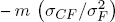 represents the hedging component of the position; it is this component that leads to minimal variance;
 represents the speculative component of the position; the operator bets on the foreseeable gains on the financial market.
NOTE.– It should be noted that according to this model, a rational operator is simultaneously a hedger and a speculator.
The reader must keep in mind that the strategy presented above is very basic as the operator takes a position on the date 0 and then waits for the results from this position on date τ; in practice, participants in the future markets regularly adjust their positions based on the changes on the spot market and the futures market.
3.7. Forward contracts
A forward contract has many similarities to a futures contract: when it is concluded, on a date 0, an operator commits to delivering a certain quantity of the goods, at a certain price, on a date T to another operator who commits to taking a delivery of the merchandise and paying for it on the date T .
A forward does, however, differ from a futures on several points:
- – fundamentally, a forward is meant to be executed and, therefore, ends in a physical delivery, while in the large majority of cases operators in a futures contract close their position before the maturity date, cashing in their gains or losses on the financial market, but do not proceed to an actual physical delivery;
- – a forward contract does not give rise to any physical or financial flow between 0 and T. On the date T, and in the case of a physical delivery (which represents the majority of the cases), the underlying entity with a value CT = FT,T is delivered against the payment of F0,T. In the case of a cash settlement, the losing party pays the margin |FT,T − F0,T| to the winner, on the date T;
- – a forward contract is negotiated over the counter and is not generally standardized.
Forward contracts are well adapted for direct transactions between producers and transformers: they allow producers to secure their openings, while guaranteeing transformers a supply. This mutual guarantee is, however, altered by the risk of a counterparty; if either of the two contracting parties does not respect their commitment, it could be difficult for the other party to obtain compensation. Forwards are, for example, very common between potato producers and industrial producers of frozen fries. Contractualization is also widespread in tinned vegetables:
“Contractualization in our field is not something that just happened. […] There is a contract template, however the contractualization is carried out between each industrialist and producer organizations, for a duration of one year. Our contracts establish the price, the quality, or again the schedule for harvesting etc. We have, on the one hand, companies that need commodities, and on the other hand, farmers who need to make a choice in their rotation. It is essential that all of this be clear. These negotiations are not always easy, but to build a lasting relationship there must be a relationship of trust”3.
3.8. The pricing of futures and forwards
This section examines the outline of an article by Fischer Black [BLA 76]; the notations used are those from the article. Fischer Black asks two simple questions: what is the value of a futures contract? What is the value of a forward contract?4 We will use Black’s discussion as it offers a greater understanding of what futures contracts are and their uniqueness in economics.
3.8.1. The bases of the Black model
The spot price of a commodity at the instant t is denoted by ct. xt,T, or more simply x, denotes the price at which a future contract with the maturity date T is traded at the time t, with t ≤ T ; x is the price upon which at least two operators have agreed. It is, thus, a market price resulting from a negotiation. In general:
Equation [3.1] must be read as a limit case: if we commit today to a future contract maturing immediately, rationality imposes that this be done at the market price as it would be aberrant for either the seller to commit to a lower price or for a buyer to commit to a higher price than the price that prevails at that point in time. This general relationship is all the more important when t = T as it signifies that the basis cancels itself out, a necessary condition for the optimal hedge.
The value of a forward is denoted by v and the value of a futures is denoted by u. The word “value” here signifies that a forward or a futures will lead to positive or negative financial flows for the operators involved in these contracts. The flows resulting from a contract are in opposite directions for the buyer and seller of this contract. Black ignores commissions and taxes. To simplify the discussion, u and v will be considered as the value of the contract for the buyer, that is the operator taking the long position, to use the jargon of the commodity markets. The interest rates are assumed to be zero and it is, therefore, not necessary to update the financial flows. Using x to denote the price at which a futures contract is concluded, we can write that the value of a forward is:
Black’s notation, which is extremely concise, must be explained: the pair (x, t) of the quadruplet (x, t, x, T) designates the fact that a futures contract was concluded at a price x at the time t; the pair (x, T) from the quadruplet (x, t, x, T) designates the fact that a forward contract with the maturity date T was concluded at the price x. Equation [3.2] must thus be read as: v (x, t, x, T) = (x, t) − (x, T) = (price of the futures) - (price of the forward). In concrete terms, this formula states that a buyer who has committed to a forward contract has made a good deal if the price of the futures contract becomes higher than that of the forward. This is because in this case the buyer has committed to a lower price than the market price.
At the time that it is concluded, the price of a forward is always equal to the price of a future. Thus, the difference in values is zero. If this were not the case, an easy arbitrage opportunity would immediately emerge. For example, if a forward contract could be concluded for delivery at a price c < x, it would be enough to take the long position on the futures contract and the short position on the forward contract to yield certain gain.5 Symmetric arbitrage can clearly be formulated in the case where c > x. Equation [3.2] also reflects a reality of derivative markets, namely that a futures can be used as a forward by taking a position on any date t, maintaining it till maturity and proceeding with a physical delivery upon maturity. It is, thus, normal that when a forward contract is concluded, it is concluded at the same price as a futures contract, because this can be used as a forward.6
c denotes the price that the buyer of a forward contract commits to paying for the underlying asset at the time T. Of course, the seller has committed to delivering the underlying entity at this same price, c, however, let us recall that for convenience’s sake, the value of the contract is studied solely from the buyer’s point of view. As soon as the market price changes and thus differs from c, the value of the forward contract increases for one party and decreases for the other. For the buyer of a forward, the value changes as follows:
This system of equations can be rewritten as:
The value of a forward is measured by the difference between the price at which it was concluded and the price of the futures contract. The price at which the forward was concluded is constant; on the contrary, the price of the futures contract changes very frequently and, thus, the value of the forward contract, as defined by Black, changes at the same rate as the price of the futures contract. Formally, the value of the forward depends directly on x and, therefore, on ct (the price of the underlying support) as xt,t ≡ ct. It also depends on c, the price at which the delivery must take place. At the time of maturity, T :
In summary, at the time that it is concluded, a forward contract has a null value. Consequently, depending on the change in the price of the support, the contract will gain or lose value, but it is only at the time of maturity that it results in a financial flow, which may be positive or negative, depending on the position taken by the operator. This point can be easily understood. However, the next part concerning futures is more difficult. We reproduce here, almost verbatim, a crucial passage from Fischer Black: the contract is rewritten each day with a new exercise price, c, equal to x, the price of the corresponding futures. A futures contract can be compared to a series of forward contracts. Every day when the markets close the contract signed the previous day is executed and a new contract is concluded with an exercise price that is equal to the price of the futures contract with the same maturity date.
Equation [3.2] shows that a forward contract concluded at the price of a futures contract is of null value at the time that it is signed. Moreover, a futures contract results in a margin call every day, payable or receivable, depending on the change in price with respect to the previous day’s closing price. Once the margin call is collected or paid, the value of a futures is reset to zero. It becomes possible to compare a futures contract to a series of forward contracts rewritten after each closing of the market, with these forward contracts being of null value at the instant that they are rewritten. In other words, the value of a futures is reset to zero on a daily basis following the payment of the margin calls. This can be summarized in the following equation:
Let us highlight the fact that equation [3.5] is valid only for the closing of the market, after the margin calls have been paid. Before the closing, the futures contract gains or loses value like the corresponding forward. The paradox in equation [3.5] can be easily explained: every day, after the margin calls are paid, a future has null value, but since the operator has taken a position and has not closed this position, they have accumulated margin calls that translate into a gain or a loss over the duration of the position being held. In other terms, gains or losses accumulate over the period that a position is maintained: even if the value of a futures is reset to zero every day after the margin calls, the position that the futures allowed the operator to take generates results.
The Black model formalizes what we presented in section 3.3.2, but also goes further. This model makes it possible to highlight the economic uniqueness of futures and forwards: the value of these financial instruments change constantly depending on the changes in the price of the underlying support. More surprisingly, every day after the payment of the margin calls that follow the closing of the markets, a futures contract has a null value until the market reopens again. This result is surprising because expression [3.5] only takes into account the financial flows that have already been paid; it does not take into account the flows expected by the operators who sign a future contract. Another remarkable result, to which we will return in section 4.1.2 can be deduced from this expression: futures markets would not exist in the absence of uncertainty. It is uncertainty that creates the need for futures markets.
3.8.2. The dynamic of futures prices
The manner in which futures prices form and evolve is a central question in financial economics and we will return to it repeatedly in the remaining sections of the text. We will turn here to the broad outlines of the analysis that Black proposed, as this analysis yields several important results.
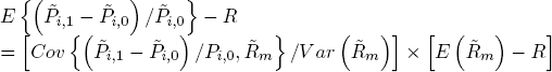
Black hypothesized that it was possible to work within the framework of the Capital Asset Pricing Model, which meant that the value of any asset included in an investment portfolio could be characterized with the help of a few simple parameters. Futures contracts make up one class of assets among others and can, therefore, be characterized in the same generic manner as any other financial asset [DUS 73]. Within the framework of the CAPM, the expected return from an asset i is given by the expression:
In this expression ![]() is the return on the asset i, expressed as a fraction of its initial value; R is the short-term rate of interest and Rm is the return from the market portfolio that contains all of the assets. R is, in fact, a risk-free rate, while
is the return on the asset i, expressed as a fraction of its initial value; R is the short-term rate of interest and Rm is the return from the market portfolio that contains all of the assets. R is, in fact, a risk-free rate, while ![]() represents the return that we may expect if we invest in the totality of risky assets. Taxes and transaction costs are assumed to be zero. The coefficient βi is defined as:
represents the return that we may expect if we invest in the totality of risky assets. Taxes and transaction costs are assumed to be zero. The coefficient βi is defined as:
If βi > 1, the variations in the asset i are greater than the variations on the market; we then consider that investing in the asset i is riskier than investing across the market as a whole. Conversely, if βi < 1, the asset i is considered to be less risky but the expected returns will be lower.
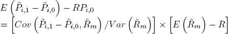
Equation [3.6] cannot be directly used for a futures contract because its initial value is null. Thus, the concept of return is meaningless here. Black rewrites this equation so that it can be expressed in monetary units and not in percentage. If the asset i, with a non-zero initial price, does not result in any financial flow over an investment period, then its return is: the terminal price, denoted by ![]() , minus the initial price
, minus the initial price ![]() , the whole divided by the initial price.
, the whole divided by the initial price.
Equation [3.6] is rewritten as:
Upon multiplying by Pi,0 we have:
At the beginning of the period, a futures has a value of zero, thus Pi,0 = 0; at the end of the period, and before paying the margin calls, the value of a contract is equal to the change in price of the futures contract over the period. The variation of the futures price over the period is denoted by ![]() . Hence:
. Hence:
By now using a value β*, defined as the “dollar beta” [BLA 76], we obtain:
This equation shows that the expectation of variations in a futures price may be positive, negative or null. It is zero notably when ![]() . This result is very important: the variations in price may be the source of a financial return, thus, futures contracts may be investment supports, not only hedging tools. From a theoretical point of view, Black opens up the path to what we today call the financialization of futures markets, which will be discussed in detail in Chapter 4.
. This result is very important: the variations in price may be the source of a financial return, thus, futures contracts may be investment supports, not only hedging tools. From a theoretical point of view, Black opens up the path to what we today call the financialization of futures markets, which will be discussed in detail in Chapter 4.
3.9. Commodity swaps
3.9.1. Definition and example
In finance, a swap is used to designate a contract through which two parties exchange two series of financial flows. In a commodity swap, one of the operators (Bank B) commits to paying, at n regular intervals, a financial flow that depends on the price observed on a market for each maturity date. In return, the other contractor (Company A) will pay a fixed flow, defined at the time the contract is signed. In this example, Company A will win if the series of spot prices is such that the variable flows they pay are, on average, lower than the fixed flows they will receive.
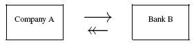
Figure 3.2. Swap of a series of fixed flows (from A to B) against a series of variable flows (from B to A)
A fixed flux is usually represented by a single-headed arrow and a variable flux by an arrow with two heads. A very important point: each flow is repeated at regular intervals for the full duration of the swap. A commodity swap does not usually lead to a physical delivery. To be on the safe side, we will qualify that we have never heard of such a contract. Having said this, the contractor enjoys quite a bit of freedom and thus, a swap with a physical delivery is not impossible. A few clarifications must be made: first of all, the variable price of the commodity is called the floating price and the fixed price is called the constant flow, paid for the full duration of the swap. Further, a swap is signed for a limited period, thus the number of flows and their periodicity are part of the terms of the contract. It can be easily understood that, depending on the changes in the support, the swap will gain in or lose value for one or the other of the parties. For example, if the price of the commodity rises, then the party paying the fixed flow is in a winning position, while the party paying the variable flow loses.
Commodity swaps are very widely used. In practice, they are proposed by specialized actors, often banks. An operator who seeks to hedge, an airline company, for instance, that must regularly buy jet fuel, will easily find a range of propositions for swaps. The negotiation of a swap is, in fact, a rapid process as the contracts are heavily standardized and the terms of the contract are not negotiated line by line. Consequently, if a price is suitable to one hedger, a few “clicks” suffice for the contract to be concluded and to come into effect. Once the swap is signed, the hedger is protected against variations in price, while the seller of the hedge becomes exposed to this risk. In a very general manner, the seller of the swap will themselves engage in another swap that will allow them to diminish or cancel out their risk. Of course, a bank simultaneously engages in many swaps only if the revenue from the flows that it receives and pays out allows it to realize a margin that is deemed sufficient. Indeed, banks – or other specialized operators – normally take few risks by combining diverse operations where the revenue from the flow is positive and near-certain.
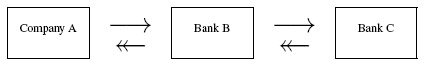
Figure 3.3. A double swap makes it possible for Bank B to take a position that is almost risk free
In this case, Bank B pays a variable flow to Company A, but it receives another variable flow, indexed on the same commodity, from Bank C. The two fixed flows are known. B is, therefore, no longer exposed to the risk of fluctuations in the price of the commodities. Of course, B will only engage in this double operation if the arithmetic sum of the flows is positive. Nevertheless, the operation is not, strictly speaking, completely risk free for B as one or the other of its counterparties may default. As this is an OTC operation, a completion of the transactions is not guaranteed by a CH. We will see, in Chapter 8, that these incompressible risks resulting from OTC operations present regulation problems.
This very simple example also makes it possible to highlight another crucial point: it is almost certain that Bank C will itself be engaged in other swaps. We can thus see that swaps constitute a sort of chain in which multiple actors are involved; if one of these actors defaults, the consequences may affect all actors along the chain, resulting in the problems regulators face.
3.9.2. Pricing a swap
A commodity swap generates random financial flows. Both on the theoretical level as well as the operational terms that aid in decision making, it is necessary to evaluate a contract before signing it. The basic principle of pricing a swap is extremely simple and can be summarized in an expression as follows:

V0 designates the value of the swap at the time it was concluded, on the date t = 0, T is the maturity date of the swap, c is the fixed flow amount, ![]() is the random flow and r is the discount rate. In this formula, V0 is estimated from the point of view of the party that receives the fixed flows and pays the variable flows. The value of the swap for the seller is, clearly, the opposite of V0.7
is the random flow and r is the discount rate. In this formula, V0 is estimated from the point of view of the party that receives the fixed flows and pays the variable flows. The value of the swap for the seller is, clearly, the opposite of V0.7
Chapter written by Joël PRIOLON.