Chapter 4. Multiple Regression: Rushing Yards Over Expected
In the previous chapter, you looked at rushing yards through a different lens, by controlling for the number of yards needed to gain for a first down or a touchdown. You found that common sense prevails; the more yards a team needs to earn for a first down or a touchdown, the easier it is to gain yards on the ground. This tells you that adjusting for such things is going to be an important part of understanding running back play.
A limitation of simple linear regression is that you will have more than one important variable to adjust for in the running game. While distance to first down or touchdown matters a great deal, perhaps the down is important as well. A team is more likely to run the ball on first down and 10 yards to go than it is to run the ball on third down and 10 yards to go, and hence the defense is more likely to be more geared up to stop the run on the former than the latter.
Another example is point differential. The score of the game influences the expectation in multiple ways, as a team that is ahead by a lot of points will not crowd the line of scrimmage as much as a team that is locked into a close game with its opponent. In general, a plethora of variables need to be controlled for when evaluating a football play. The way we do this is through multiple linear regression.
Definition of Multiple Linear Regression
We know that running the football isn’t affected by just one thing, so we need to build a model that predicts rushing yards, but includes more features to account for other things that might affect the prediction. Hence, to build upon Chapter 3, we need multiple regression.
Multiple regression estimates for the effect of several (multiple) predictors on a single response by using a linear combination (or regression) of the predictor variables. Chapter 3 presented simple linear regression, which is a special case of multiple regression. In a simple linear regression, two parameters exist: an intercept (or average value) and a slope. These model the effect of a continuous predictor on the response. In Chapter 3, the Python/R formula for your simple linear regression had rushing yards predicted by an intercept and yards to go: rushing_yards ~ 1 + ydstogo.
However, you may be interested in multiple predictor variables. For example, consider the multiple regression that corrects for down when estimating expected rushing yards. You would use an equation (or formula) that predicts rushing yards based on yards to go and down: rushing_yards ~ ydstogo + down. Yards to go is an example of a continuous predictor variable. Informally, think of continuous predictors as numbers such as a players’ weights, like 135, 302, or 274. People sometimes use the term slope for continuous predictor variables. Down is an example of a discrete predictor variable. Informally, think of discrete predictors as groups or categories such as position (like running back or quarterback). By default, the formula option in statsmodels and base R treat discrete predictors as contrasts.
Let’s dive into the example formula, rushing_yards ~ ydstogo + down. R would estimate an intercept for the lowest (or alphabetically first) down and then the contrast, or difference, for the other downs. For example, four predictors would be estimated: an intercept that is the mean rushing_yards for yards to go, a contrast for second downs compared to first down, a contrast for third downs compared to first down, and a contrast for fourth downs compared to first down. To see this, look at the design matrix, or model matrix, in R (Python has similar features that are not shown here). First, create a demonstration dataset:
## Rlibrary(tidyverse)demo_data_r<-tibble(down=c("first","second"),ydstogo=c(10,5))
Then, create a model matrix by using the formula’s righthand side and the model.matrix() function:
## Rmodel.matrix(~ydstogo+down,data=demo_data_r)
Resulting in:
  (Intercept) ydstogo downsecond
1           1      10          0
2           1       5          1
attr(,"assign")
[1] 0 1 2
attr(,"contrasts")
attr(,"contrasts")$down
[1] "contr.treatment"
Notice that the output has three columns: an intercept, a slope for ydstogo, and a contrast for second down (downsecond).
However, you can also estimate an intercept for each down by using a -1, such as rushing_yards ~ ydstogo + down -1. This would estimate four predictors: an intercept for first down, an intercept for second down, an intercept for third down, and an intercept for fourth down. Use R to look at the example model matrix:
## Rmodel.matrix(~ydstogo+down-1,data=demo_data_r)
Resulting in:
  ydstogo downfirst downsecond
1      10         1          0
2       5         0          1
attr(,"assign")
[1] 1 2 2
attr(,"contrasts")
attr(,"contrasts")$down
[1] "contr.treatment"
Notice that you have the same number of columns as before, but each down has its own column.
Warning
Computer languages such as Python and R get confused by some groups
such as down. The computer tries to treat these predictors as continuous,
such as the numbers 1, 2, 3, and 4 rather than first down,
second down, third down, and fourth down. In pandas you will
change down to be a string (str), and in R, you will change down to
be a character.
The formula for multiple regression allows for many discrete and continuous predictors. When multiple discrete predictors are present, such as down + team, the first variable (down, in this case) can either be estimated as an intercept or contrast parameters. All other discrete predictors are estimated as contrasts, with the first groupings treated as part of the intercept. Rather than getting caught up in thinking about slopes and intercepts, you can use the term coefficients to describe the estimated predictor variables for multiple regression.
Exploratory Data Analysis
In the case of rushing yards, you’re going to use the following variables as features in the multiple linear regression model: down (down), distance (ydstogo), yards to go to the endzone (yardline_100), run location (run_location), and score differential (score_differential). Other variables could also be used, of course, but for now you’re using these variables in large part because they all affect rushing yards in one way or another.
First, load in the data and packages you will be using, filter for only the run data (as you did in Chapter 3), and remove plays that were not a regular down. Do this with Python:
importpandasaspdimportnumpyasnpimportnfl_data_pyasnflimportstatsmodels.formula.apiassmfimportmatplotlib.pyplotaspltimportseabornassnsseasons=range(2016,2022+1)pbp_py=nfl.import_pbp_data(seasons)pbp_py_run=pbp_py.query('play_type == "run" & rusher_id.notnull() &'+"down.notnull() & run_location.notnull()").reset_index()pbp_py_run.loc[pbp_py_run.rushing_yards.isnull(),"rushing_yards"]=0
Or with R:
library(tidyverse)library(nflfastR)pbp_r<-load_pbp(2016:2022)pbp_r_run<-pbp_r|>filter(play_type=="run"&!is.na(rusher_id)&!is.na(down)&!is.na(run_location))|>mutate(rushing_yards=ifelse(is.na(rushing_yards),0,rushing_yards))
Next, let’s create a histogram for down and rushing yards gained with Python in Figure 4-1:
## Python# Change theme for chaptersns.set_theme(style="whitegrid",palette="colorblind")# Change down to be an integerpbp_py_run.down=pbp_py_run.down.astype(str)# Plot rushing yards by downg=sns.FacetGrid(data=pbp_py_run,col="down",col_wrap=2);g.map_dataframe(sns.histplot,x="rushing_yards");plt.show();

Figure 4-1. Histogram of rushing yards by downs with seaborn
Or, Figure 4-2 with R:
## R# Change down to be an integerpbp_r_run<-pbp_r_run|>mutate(down=as.character(down))# Plot rushing yards by downggplot(pbp_r_run,aes(x=rushing_yards))+geom_histogram(binwidth=1)+facet_wrap(vars(down),ncol=2,labeller=label_both)+theme_bw()+theme(strip.background=element_blank())

Figure 4-2. Histogram of rushing yards by downs with ggplot2
This is interesting, as it looks like down decreases rushing yards. However, the data has a confounder, which is that rushes often happen on late downs with smaller distances. Let’s look at only situations where ydstogo == 10. In Python, create Figure 4-3:
## Pythonsns.boxplot(data=pbp_py_run.query("ydstogo == 10"),x="down",y="rushing_yards");plt.show()

Figure 4-3. Boxplot of rushing yards by downs for plays with 10 yards to go (seaborn)
Or with R, create Figure 4-4:
## Rpbp_r_run|>filter(ydstogo==10)|>ggplot(aes(x=down,y=rushing_yards))+geom_boxplot()+theme_bw()

Figure 4-4. Boxplot of rushing yards by downs for plays with 10 yards to go (ggplot2)
OK, now you see what you expect. This is an example of Simpson’s paradox: including an extra, third grouping variable changes the relationship between the two other variables. Nonetheless, it’s clear that down affects the rushing yards on a play and should be accounted for. Similarly, let’s look at yards to the endzone in seaborn with Figure 4-5 (and change the transparency with scatter_kws={'alpha':0.25} and the regression line color with line_kws={'color': 'red'}):
## Pythonsns.regplot(data=pbp_py_run,x="yardline_100",y="rushing_yards",scatter_kws={"alpha":0.25},line_kws={"color":"red"});plt.show();

Figure 4-5. Scatterplot with linear trendline for ball position (yards to go to the endzone) and rushing yards from a play (seaborn)
Or with R, create Figure 4-6 (and change the transparency with alpha = 0.25 to help you see the overlapping points):
## Rggplot(pbp_r_run,aes(x=yardline_100,y=rushing_yards))+geom_point(alpha=0.25)+stat_smooth(method="lm")+theme_bw()

Figure 4-6. Scatterplot with linear trendline for ball position (yards to go to the endzone) and rushing yards from a play (ggplot2)
This doesn’t appear to do much, but let’s look at what happens after you bin and average with Python:
## Pythonpbp_py_run_y100=pbp_py_run.groupby("yardline_100").agg({"rushing_yards":["mean"]})pbp_py_run_y100.columns=list(map("_".join,pbp_py_run_y100.columns))pbp_py_run_y100.reset_index(inplace=True)
Now, use these results to create Figure 4-7:
sns.regplot(data=pbp_py_run_y100,x="yardline_100",y="rushing_yards_mean",scatter_kws={"alpha":0.25},line_kws={"color":"red"});plt.show();

Figure 4-7. Scatterplot with linear trendline for ball position and rushing yards for data binned by yard (seaborn)
Or with R, create Figure 4-8:
## Rpbp_r_run|>group_by(yardline_100)|>summarize(rushing_yards_mean=mean(rushing_yards))|>ggplot(aes(x=yardline_100,y=rushing_yards_mean))+geom_point()+stat_smooth(method="lm")+theme_bw()

Figure 4-8. Scatterplot with linear trendline for ball position and rushing yards for data binned by yard (ggplot2)
Figures 4-7 and 4-8 show some football insight. Running plays with less than about 15 yards to go are limited by distance because there is limited distance to the endzone and tougher red-zone defense. Likewise, plays with more than 90 yards to go take the team out of its own end zone. So, defense will be trying hard to force a safety, and offense will be more likely to either punt or play conservatively to avoid allowing a safety.
Here you get a clear positive (but nonlinear) relationship between average rushing yards and yards to go to the endzone, so it benefits you to include this feature in the models. In “Assumption of Linearity”, you can see what happens to the model if values less than 15 yards or greater than 90 yards are removed. In practice, more complicated models can effectively deal with these nonlinearities, but we save that for a different book. Now, you look at run location with Python in Figure 4-9:
## Pythonsns.boxplot(data=pbp_py_run,x="run_location",y="rushing_yards");plt.show();

Figure 4-9. Boxplot of rushing yards by run location (seaborn)
Or with R in Figure 4-10:
## Rggplot(pbp_r_run,aes(run_location,rushing_yards))+geom_boxplot()+theme_bw()

Figure 4-10. Boxplot of rushing yards by run location (ggplot2)
Not only are the means/medians slightly different here, but the variances/interquartile ranges also appear to vary, so keep them in the models. Another comment about the run location is that the 75th percentile in each case is really low. Three-quarters of the time, regardless of whether a player goes left, right, or down the middle, he goes 10 yards or less. Only in a few rare cases do you see a long rush.
Lastly, look at score differential, using the binning and aggregating you used for yards to go to the endzone in Python:
## Pythonpbp_py_run_sd=pbp_py_run.groupby("score_differential").agg({"rushing_yards":["mean"]})pbp_py_run_sd.columns=list(map("_".join,pbp_py_run_sd.columns))pbp_py_run_sd.reset_index(inplace=True)
Now, use these results to create Figure 4-11:
## Pythonsns.regplot(data=pbp_py_run_sd,x="score_differential",y="rushing_yards_mean",scatter_kws={"alpha":0.25},line_kws={"color":"red"});plt.show();

Figure 4-11. Scatterplot with linear trendline for score differential and rushing yards, for data binned by score differential (seaborn)
Or in R, create Figure 4-12:
## Rpbp_r_run|>group_by(score_differential)|>summarize(rushing_yards_mean=mean(rushing_yards))|>ggplot(aes(score_differential,rushing_yards_mean))+geom_point()+stat_smooth(method="lm")+theme_bw()

Figure 4-12. Scatterplot with linear trendline for score differential and rushing yards, for data binned by score differential (ggplot2)
You can see a clear negative relationship, as hypothesized previously. Hence you will leave score differential in the model.
Tip
When you see code for plots in this book, think about how you would want to improve the plots. Also, look at the code, and if you do not understand some arguments, search and figure out how to change the plotting code. The best way to become a better data plotter is to explore and create your own plots.
Applying Multiple Linear Regression
Now, apply the multiple linear regression to rederive rushing yards over expected (RYOE). In this section, we gloss over steps that are covered in Chapter 3.
First, fit the model. Then save the calculated residuals as the RYOE. Recall that residuals are the difference between the value predicted by the model and the value observed in the data. This could be calculated directly by taking the observed rushing yards and subtracting the predicted rushing yards from the model. However, residuals are commonly used in statistics, and Python and R both include residuals as part of the model’s fit. This derivation differs from the method in Chapter 3 because you have created a more complicated model.
The model predicts rushing_yards by creating the following:
-
An intercept (
1) -
A term contrasting the second, third, and fourth downs to the first down (
down) -
A coefficient for
ydstogo -
An interaction between
ydstogoanddownthat estimates aydstogocontrast for eachdown(ydstogo:down) -
A coefficient for yards to go to the endzone (
yardline_100) -
The location of the running play on the field (
run_location) -
The difference between each team’s scores (
score_differential)
Note
Multiple approaches exist for using formulas to indicate interactions. The
longest, but most straightforward approach for our example
would be down + ydstogo + as.factor(down):ydstogo. This
may be abbreviated as down * ydstogo. Thus, the example formula, rushing_yards ~ 1 + down + ydstogo + down:ydstogo + yardline_100 + run_location + score_differential,
could be written as rushing_yards ~ down * ydstogo + yardline_100 + run_location + score_differential
and saves writing three terms.
In Python, fit the model with the statsmodels package; then save the residuals as RYOE:
## Pythonpbp_py_run.down=pbp_py_run.down.astype(str)expected_yards_py=smf.ols(data=pbp_py_run,formula="rushing_yards ~ 1 + down + ydstogo + "+"down:ydstogo + yardline_100 + "+"run_location + score_differential").fit()pbp_py_run["ryoe"]=expected_yards_py.resid
Note
We include line breaks in our code to make it fit on the pages of this book. For example, in Python, we use the string "rushing_yards ~ 1 + down + ydstogo + " followed by + and then a line break. Then, each of the next two strings, "down:ydstogo + yardline_100 + " and "run_location + score_differential" gets its own line breaks, and we then use the + character to add the strings together. These line breaks are not required but help make the code look better to human eyes and ideally be more readable.
Likewise, fit the model in, and save the residuals as RYOE in R:
## Rpbp_r_run<-pbp_r_run|>mutate(down=as.character(down))expected_yards_r<-lm(rushing_yards~1+down+ydstogo+down:ydstogo+yardline_100+run_location+score_differential,data=pbp_r_run)pbp_r_run<-pbp_r_run|>mutate(ryoe=resid(expected_yards_r))
Now, examine the summary of the model in Python:
## Python(expected_yards_py.summary())
Resulting in:
                            OLS Regression Results
==============================================================================
Dep. Variable:          rushing_yards   R-squared:                       0.016
Model:                            OLS   Adj. R-squared:                  0.016
Method:                 Least Squares   F-statistic:                     136.6
Date:                Sun, 04 Jun 2023   Prob (F-statistic):          3.43e-313
Time:                        09:36:43   Log-Likelihood:            -2.9764e+05
No. Observations:               91442   AIC:                         5.953e+05
Df Residuals:                   91430   BIC:                         5.954e+05
Df Model:                          11
Covariance Type:            nonrobust
===============================================================================
                  coef         std err     t       P>|t|       [0.025   0.975]
------------------------------------------------------------------------------
Intercept          1.6085      0.136     11.849      0.000      1.342   1.875
down[T.2.0]        1.6153      0.153     10.577      0.000      1.316   1.915
down[T.3.0]        1.2846      0.161      7.990      0.000      0.969   1.600
down[T.4.0]        0.2844      0.249      1.142      0.254     -0.204   0.773
run_location[T.middle]
                  -0.5634      0.053    -10.718      0.000     -0.666  -0.460
run_location[T.right]
                  -0.0382      0.049     -0.784      0.433     -0.134   0.057
ydstogo            0.2024      0.014     14.439      0.000      0.175   0.230
down[T.2.0]:ydstogo
                  -0.1466      0.016     -8.957      0.000     -0.179  -0.115
down[T.3.0]:ydstogo
                  -0.0437      0.019     -2.323      0.020     -0.081  -0.007
down[T.4.0]:ydstogo
                   0.2302      0.090      2.567      0.010      0.054   0.406
yardline_100       0.0186      0.001     21.230      0.000      0.017   0.020
score_differential
                  -0.0040      0.002     -2.023      0.043     -0.008  -0.000
==============================================================================
Omnibus:                    80510.527   Durbin-Watson:                   1.979
Prob(Omnibus):                  0.000   Jarque-Bera (JB):          3941200.520
Skew:                           4.082   Prob(JB):                         0.00
Kurtosis:                      34.109   Cond. No.                         838.
==============================================================================

Notes:
[1] Standard Errors assume that the covariance matrix of the errors
is correctly specified.
Or examine the summary of the model in R:
## R(summary(expected_yards_r))
Resulting in:
Call:
lm(formula = rushing_yards ~ 1 + down + ydstogo + down:ydstogo +
    yardline_100 + run_location + score_differential, data = pbp_r_run)

Residuals:
    Min      1Q  Median      3Q     Max
-32.233  -3.130  -1.173   1.410  94.112

Coefficients:
                    Estimate Std. Error t value Pr(>|t|)
(Intercept)         1.608471   0.135753  11.849  < 2e-16 ***
down2               1.615277   0.152721  10.577  < 2e-16 ***
down3               1.284560   0.160775   7.990 1.37e-15 ***
down4               0.284433   0.249106   1.142   0.2535
ydstogo             0.202377   0.014016  14.439  < 2e-16 ***
yardline_100        0.018576   0.000875  21.230  < 2e-16 ***
run_locationmiddle -0.563369   0.052565 -10.718  < 2e-16 ***
run_locationright  -0.038176   0.048684  -0.784   0.4329
score_differential -0.004028   0.001991  -2.023   0.0431 *
down2:ydstogo      -0.146602   0.016367  -8.957  < 2e-16 ***
down3:ydstogo      -0.043703   0.018814  -2.323   0.0202 *
down4:ydstogo       0.230179   0.089682   2.567   0.0103 *
---
Signif. codes:  0 '***' 0.001 '**' 0.01 '*' 0.05 '.' 0.1 ' ' 1

Residual standard error: 6.272 on 91430 degrees of freedom
Multiple R-squared:  0.01617,   Adjusted R-squared:  0.01605
F-statistic: 136.6 on 11 and 91430 DF,  p-value: < 2.2e-16
Each estimated coefficient helps you tell a story about rushing yards during plays:
-
Running plays on the second down (
down[T.2.0]in Python ordown2in R) have more expected yards per carry than the first down, all else being equal—in this case, about 1.6 yards. -
Running plays on the third down (
down[T.3.0]in Python ordown3in R) have more expected yards per carry than the first down, all else being equal—in this case, about 1.3 yards. -
The interaction term tells you that this is especially true when fewer yards to go remain for the first down (the interaction terms are all negative). From a football standpoint, this just means that second and third downs, and short yardage to go for a first down or touchdown, are more favorable to the offense running the ball than first down and 10 yards to go.
-
Conversely, running plays on fourth down have slightly more yards gained compared to first down (
down[T.4.0]in Python ordown4in R), all else being equal, but not as many as second or third down. -
As the number of yards to go increases (
ydstogo), so do the rushing yards, all else being equal, with each yard to go worth about a fifth of a yard. This is because theydstogoestimate is positive. -
As the ball is farther from the endzone, rushing plays produce slightly more yards per play (about 0.02 per yard to go to the endzone;
yardline_100). For example, even if the team has 100 yards to go, a coefficient of 0.02 means that only 2 extra yards would be rushed in the play, which doesn’t have a big impact compared to other coefficients. -
Rushing plays in the middle of the field earn about a half yard less than plays to the left, based on the contrast estimate between the middle and left side of the field (
run_location[T.middle]in Python orrun_locationmiddlein R). -
The negative
score_differentialcoefficient differs statistically from 0. Thus, when teams are ahead (have a positive score differential), they gain fewer yards per play on the average running play. However, this effect is so small (0.004) and thus not important compared to other coefficients that it can be ignored (for example, being up by 50 points would decrease the number of yards by only 0.2 per carry).
Notice from the coefficients that running to the middle of the field is harder than running to the outside, all other factors being equal. You indeed see that distance and yards to go to the first down marker and to the endzone both positively affect rushing yards: the farther an offensive player is away from the goal, the more defense will surrender to that offensive player on average.
Tip
The kableExtra package in R helps produce well-formatted tables in
R Markdown and Quarto documents as well as onscreen. You’ll need to install the package if you have not done so already.
Tables provide another way to present regression coefficients. For example, the broom package allows you to create tidy tables in R that can then be formatted by using the kableExtra package, such as Table 4-1. Specifically, with this code, take the model fit expected_yards_r and then pipe the model to extract the tidy model outputs (including the 95% CIs) by using tidy(conf.int = TRUE). Then, convert the table to a kable table and show two digits by using kbl(format = "pipe", digits = 2). Last, apply styling from the kableExtra package by using kable_styling():
## Rlibrary(broom)library(kableExtra)expected_yards_r|>tidy(conf.int=TRUE)|>kbl(format="pipe",digits=2)|>kable_styling()
| Term | estimate | std.error | statistic | p.value | conf.low | conf.high |
|---|---|---|---|---|---|---|
(Intercept) | 1.61 | 0.14 | 11.85 | 0.00 | 1.34 | 1.87 |
| 1.62 | 0.15 | 10.58 | 0.00 | 1.32 | 1.91 |
| 1.28 | 0.16 | 7.99 | 0.00 | 0.97 | 1.60 |
| 0.28 | 0.25 | 1.14 | 0.25 | -0.20 | 0.77 |
| 0.20 | 0.01 | 14.44 | 0.00 | 0.17 | 0.23 |
| 0.02 | 0.00 | 21.23 | 0.00 | 0.02 | 0.02 |
| -0.56 | 0.05 | -10.72 | 0.00 | -0.67 | -0.46 |
| -0.04 | 0.05 | -0.78 | 0.43 | -0.13 | 0.06 |
| 0.00 | 0.00 | -2.02 | 0.04 | -0.01 | 0.00 |
| -0.15 | 0.02 | -8.96 | 0.00 | -0.18 | -0.11 |
| -0.04 | 0.02 | -2.32 | 0.02 | -0.08 | -0.01 |
| 0.23 | 0.09 | 2.57 | 0.01 | 0.05 | 0.41 |
Tip
Writing about regressions can be hard, and knowing your audience and their background is key. For example, the paragraph “Notice from the coefficients…” would be appropriate for a casual blog but not for a peer-reviewed sports journal. Likewise, a table like Table 4-1 might be included in a journal article but is more likely to be included as part of a technical report or journal article’s supplemental materials. Our walk-through of individual coefficients in a bulleted list might be appropriate for a report to a client who wants an item-by-item description or for a teaching resource such as a blog or book on football analytics.
Analyzing RYOE
Just as with the first version of RYOE in Chapter 3, now you will analyze the new version of your metric for rushers. First, create the summary tables for the RYOE totals, means, and yards per carry in Python. Next, save only data from players with more than 50 carries. Also, rename the columns and sort by total RYOE:
## Pythonryoe_py=pbp_py_run.groupby(["season","rusher_id","rusher"]).agg({"ryoe":["count","sum","mean"],"rushing_yards":["mean"]})ryoe_py.columns=list(map("_".join,ryoe_py.columns))ryoe_py.reset_index(inplace=True)ryoe_py=ryoe_py.rename(columns={"ryoe_count":"n","ryoe_sum":"ryoe_total","ryoe_mean":"ryoe_per","rushing_yards_mean":"yards_per_carry"}).query("n > 50")(ryoe_py.sort_values("ryoe_total",ascending=False))
Resulting in:
      season   rusher_id      rusher  ...  ryoe_total  ryoe_per  yards_per_carry
1870    2021  00-0036223    J.Taylor  ...  471.232840  1.419376         5.454819
1350    2020  00-0032764     D.Henry  ...  345.948778  0.875820         5.232911
1183    2019  00-0034796   L.Jackson  ...  328.524757  2.607339         6.880952
1069    2019  00-0032764     D.Henry  ...  311.641243  0.807361         5.145078
1383    2020  00-0033293     A.Jones  ...  301.778866  1.365515         5.565611
...      ...         ...         ...  ...         ...       ...              ...
627     2018  00-0027029     L.McCoy  ... -208.392834 -1.294365         3.192547
51      2016  00-0027155  R.Jennings  ... -228.084591 -1.226261         3.344086
629     2018  00-0027325    L.Blount  ... -235.865233 -1.531592         2.714286
991     2019  00-0030496      L.Bell  ... -338.432836 -1.381359         3.220408
246     2016  00-0032241    T.Gurley  ... -344.314622 -1.238542         3.183453

[533 rows x 7 columns]
Next, sort by mean RYOE per carry in Python:
## Python(ryoe_py.sort_values("ryoe_per",ascending=False))
Resulting in:
      season   rusher_id        rusher ...  ryoe_total  ryoe_per  yards_per_carry
2103    2022  00-0034796     L.Jackson ...  280.752317  3.899338  7.930556
1183    2019  00-0034796     L.Jackson ...  328.524757  2.607339  6.880952
1210    2019  00-0035228      K.Murray ...  137.636412  2.596913  6.867925
2239    2022  00-0036945      J.Fields ...  177.409631  2.304021  6.506494
1467    2020  00-0034796     L.Jackson ...  258.059489  2.186945  6.415254
...      ...         ...           ... ...         ...       ...              ...
1901    2021  00-0036414       C.Akers ... -129.834294 -1.803254  2.430556
533     2017  00-0032940  D.Washington ... -105.377929 -1.848736  2.684211
1858    2021  00-0035860       T.Jones ... -100.987077 -1.870131  2.629630
60      2016  00-0027791      J.Starks ... -129.298259 -2.052353  2.301587
1184    2019  00-0034799     K.Ballage ... -191.983153 -2.594367  1.824324

[533 rows x 7 columns]
These same tables may be created in R as well:
## Rryoe_r<-pbp_r_run|>group_by(season,rusher_id,rusher)|>summarize(n=n(),ryoe_total=sum(ryoe),ryoe_per=mean(ryoe),yards_per_carry=mean(rushing_yards))|>filter(n>50)ryoe_r|>arrange(-ryoe_total)|>()
Resulting in:
# A tibble: 533 × 7
# Groups:   season, rusher_id [533]
   season rusher_id  rusher        n ryoe_total ryoe_per yards_per_carry
    <dbl> <chr>      <chr>     <int>      <dbl>    <dbl>           <dbl>
 1   2021 00-0036223 J.Taylor    332       471.    1.42             5.45
 2   2020 00-0032764 D.Henry     395       346.    0.876            5.23
 3   2019 00-0034796 L.Jackson   126       329.    2.61             6.88
 4   2019 00-0032764 D.Henry     386       312.    0.807            5.15
 5   2020 00-0033293 A.Jones     221       302.    1.37             5.57
 6   2022 00-0034796 L.Jackson    72       281.    3.90             7.93
 7   2019 00-0031687 R.Mostert   190       274.    1.44             5.83
 8   2016 00-0033045 E.Elliott   342       274.    0.800            5.14
 9   2020 00-0034796 L.Jackson   118       258.    2.19             6.42
10   2021 00-0034791 N.Chubb     228       248.    1.09             5.52
# ℹ 523 more rows
Then sort by mean RYOE per carry in R:
## Rryoe_r|>filter(n>50)|>arrange(-ryoe_per)|>()
Resulting in:
# A tibble: 533 × 7
# Groups:   season, rusher_id [533]
   season rusher_id  rusher        n ryoe_total ryoe_per yards_per_carry
    <dbl> <chr>      <chr>     <int>      <dbl>    <dbl>           <dbl>
 1   2022 00-0034796 L.Jackson    72      281.      3.90            7.93
 2   2019 00-0034796 L.Jackson   126      329.      2.61            6.88
 3   2019 00-0035228 K.Murray     53      138.      2.60            6.87
 4   2022 00-0036945 J.Fields     77      177.      2.30            6.51
 5   2020 00-0034796 L.Jackson   118      258.      2.19            6.42
 6   2017 00-0027939 C.Newton     92      191.      2.08            6.17
 7   2020 00-0035228 K.Murray     70      144.      2.06            6.06
 8   2021 00-0034750 R.Penny     119      242.      2.03            6.29
 9   2019 00-0034400 J.Wilkins    51       97.8     1.92            6.02
10   2022 00-0033357 T.Hill       95      171.      1.80            6.05
# ℹ 523 more rows
The preceding outputs are similar to those from Chapter 3 but come from a model that corrects for additional features when estimating RYOE.
When it comes to total RYOE, Jonathan Taylor’s 2021 season still reigns supreme, and now by over 100 yards over expected more than the next-best player, while Derrick Henry makes a couple of appearances again. Nick Chubb has been one of the best runners in the entire league since he was drafted in the second round in 2018, while Raheem Mostert of the 2019 NFC champion San Francisco 49ers wasn’t even drafted at all but makes the list. Ezekiel Elliott of the Cowboys and Le’Veon Bell of the Pittsburgh Steelers, New York Jets, Chiefs, and Ravens make appearances at various places: we’ll talk about them later.
As for RYOE per carry (for players with 50 or more carries in a season), Rashaad Penny’s brilliant 2021 shines again. But the majority of the players in this list are quarterbacks, like 2019 league MVP Lamar Jackson; 2011 and 2019 first-overall picks Cam Newton and Kyler Murray, respectively; and the New Orleans Saints’ Taysom Hill. Justin Fields, who had one of the best rushing seasons in the history of the quarterback position in 2022, shows up as well.
As for the stability of this metric relative to yards per carry, recall that in the previous chapter, you got a slight bump in stability though not necessarily enough to say that RYOE per carry is definitively a superior metric to yards per carry for rushers. Let’s redo this analysis:
## Python# keep only the columns neededcols_keep=["season","rusher_id","rusher","ryoe_per","yards_per_carry"]# create current dataframeryoe_now_py=ryoe_py[cols_keep].copy()# create last-year's dataframeryoe_last_py=ryoe_py[cols_keep].copy()# rename columnsryoe_last_py.rename(columns={'ryoe_per':'ryoe_per_last','yards_per_carry':'yards_per_carry_last'},inplace=True)# add 1 to seasonryoe_last_py["season"]+=1# merge togetherryoe_lag_py=ryoe_now_py.merge(ryoe_last_py,how='inner',on=['rusher_id','rusher','season'])
Then examine the correlation for yards per carry:
## Pythonryoe_lag_py[["yards_per_carry_last","yards_per_carry"]].corr()
Resulting in:
                      yards_per_carry_last  yards_per_carry
yards_per_carry_last              1.000000         0.347267
yards_per_carry                   0.347267         1.000000
Repeat with RYOE:
## Pythonryoe_lag_py[["ryoe_per_last","ryoe_per"]].corr()
Resulting in:
               ryoe_per_last  ryoe_per
ryoe_per_last       1.000000  0.373582
ryoe_per            0.373582  1.000000
These calculations may also be done using R:
## R# create current dataframeryoe_now_r<-ryoe_r|>select(-n,-ryoe_total)# create last-year's dataframe# and add 1 to seasonryoe_last_r<-ryoe_r|>select(-n,-ryoe_total)|>mutate(season=season+1)|>rename(ryoe_per_last=ryoe_per,yards_per_carry_last=yards_per_carry)# merge togetherryoe_lag_r<-ryoe_now_r|>inner_join(ryoe_last_r,by=c("rusher_id","rusher","season"))|>ungroup()
Then select the two yards-per-carry columns and examine the correlation:
## Rryoe_lag_r|>select(yards_per_carry,yards_per_carry_last)|>cor(use="complete.obs")
Resulting in:
                     yards_per_carry yards_per_carry_last
yards_per_carry             1.000000             0.347267
yards_per_carry_last        0.347267             1.000000
Repeat with the RYOE columns:
## Rryoe_lag_r|>select(ryoe_per,ryoe_per_last)|>cor(use="complete.obs")
Resulting in:
               ryoe_per ryoe_per_last
ryoe_per      1.0000000     0.3735821
ryoe_per_last 0.3735821     1.0000000
This is an interesting result! The year-to-year stability for RYOE slightly improves with the new model, meaning that after stripping out more and more context from the situation, we are indeed extracting some additional signal in running back ability above expectation. The issue is that this is still a minimal improvement, with the difference in r values less than 0.03. Additional work should interrogate the problem further, using better data (like tracking data) and better models (like tree-based models).
Tip
You have hopefully noticed that the code in this chapter and in Chapter 3 are repetitive and similar. If we were repeating code on a regular basis like this, we would write our own set of functions and place them in a package to allow us to easily reuse our code. “Packages” provides an overview of this topic.
So, Do Running Backs Matter?
This question seems silly on its face. Of course running backs, the players who carry the ball 50 to 250 times a year, matter. Jim Brown, Franco Harris, Barry Sanders, Marshall Faulk, Adrian Peterson, Derrick Henry, Jim Taylor—the history of the NFL cannot be written without mentioning the feats of great runners.
Tip
Ben Baldwin hosts a Nerd-to-Human Translator, which helps describe our word choices in this chapter. He notes, “What the nerds say: running backs don’t matter.” And then, “What the nerds mean: the results of running plays are primarily determined by run blocking and defenders in the box, not who is carrying the ball. Running backs are interchangeable, and investing a lot of resources (in the draft or free agency) doesn’t make sense.” And then he provides supporting evidence. Check out his page for this evidence and more useful tips.
However, we should note a couple of things. First, passing the football has gotten increasingly easier over the course of the past few decades. In “The Most Important Job in Sports Is Easier Than Ever Before”, Kevin Clark notes how “scheme changes, rule changes, and athlete changes” all help quarterbacks pass for more yards. We’ll add technology (e.g., the gloves the players wear), along with the adoption of college offenses and the creative ways in which they pass the football, to Kevin’s list.
In other words, the notion that “when you pass, only three things can happen (a completion, an incompletion, or an interception), and two of them are bad” doesn’t take into account the increasing rate at which the first thing (a completion) happens. Passing has long been more efficient than running (see “Exercises”), but now the variance in passing the ball has shrunk enough to prefer it in most cases to the low variance (and low efficiency) of running the ball.
In addition to the fact that running the ball is less efficient than passing the ball, whether measured through yards per play or something like expected points added (EPA), the player running the ball evidently has less influence over the outcome of a running play than previously thought.
Other factors that we couldn’t account for by using nflfastR data also work against running backs influencing their production. Eric, while he was at PFF, showed that offensive line play carried a huge signal when it came to rushing plays, using PFF’s player grades by offensive linemen on a given play.
Eric also showed during the 2021 season that the concept of a perfectly blocked run—running play where no run blocker made a negative play (such as getting beaten by a defender)—changed the outcome of a running play by roughly half of an expected point. While the running back can surely aid in the creation of a perfectly blocked play through setting up his blockers and the like, the magnitude of an individual running back’s influence is unlikely to be anywhere close to this value.
The NFL has generally caught up to this phenomenon, spending less and less as a percentage of the salary cap on running backs for the past decade plus, as Benjamin Morris shows in “Running Backs Are Finally Getting Paid What They’re Worth” from FiveThirtyEight. Be that as it may, some contention remains about the position, with some players who are said to “break the mold” getting big contracts, usually to the disappointment of their teams.
An example of a team overpaying its star running back, and likely regretting it, occurred when the Dallas Cowboys in the fall of 2019, signed Ezekiel Elliott to a six-year, $90 million contract, with $50 million in guarantees. Elliott was holding out for a new deal, no doubt giving Cowboys owner Jerry Jones flashbacks to 1993, when the NFL’s all-time leading rusher Emmitt Smith held out for the first two games for the defending champion Cowboys. The Cowboys, after losing both games without Smith, caved to the star’s demands, and he rewarded them by earning the NFL’s MVP award during the regular season. He finished off the season by earning the Super Bowl MVP as well, helping lead Dallas to the second of its three championships in the mid-’90s.
Elliott had had a similar start to his career as Smith, leading the NFL in rushing yards per game in each of his first three seasons leading up to his holdout, and leading the league in total rushing yards during both seasons when he played the full year (Elliott was suspended for parts of the 2017 season). The Cowboys won their division in 2016 and 2018, and won a playoff game, only its second since 1996, in 2018.
As predicted by many in the analytics community, Zeke struggled to live up to the deal, with his rushing yards per game falling from 84.8 in 2019, to 65.3 in 2020, and flattening out to 58.9 and 58.4 in 2021 and 2022, respectively. Elliott’s yards per carry in 2022 fell beneath 4.0 to 3.8, and he eventually lost his starting job—and job altogether—to his backup Tony Pollard, in the 2023 offseason.
Not only did Elliott fail to live up to his deal, but his contract was onerous enough that the Cowboys had to jettison productive players like wide receiver Amari Cooper to get under the salary cap, a cascading effect that weakened the team more than simply the negative surplus play of a running back could.
An example of a team holding its ground, and likely breathing a sigh of relief, occurred in 2018. Le’Veon Bell, who showed up in “Analyzing RYOE”, held out of training camp and the regular season for the Pittsburgh Steelers in a contract dispute, refusing to play on the franchise tag—an instrument a team uses to keep a player around for one season at the average of the top five salaries at their respective position. Players, who usually want longer-term deals, will often balk at playing under this contract type, and Bell—who gained over 5,000 yards on the ground during his first four years with the club, and led the NFL in touches in 2017 (carries and receptions)—was one such player.
The problem for Bell was that he was easily replaced in Pittsburgh. James Conner, a cancer survivor from the University of Pittsburgh selected in the third round of the 2017 NFL Draft, rushed for over 950 yards, at 4.5 yards per carry (Bell’s career average was 4.3 as a Steeler), with 13 total touchdowns—earning a Pro Bowl berth.
Bell was allowed to leave for the lowly Jets the following year, where he lasted 17 games and averaged just 3.3 yards per carry, scoring just four times. He did land with the Kansas City Chiefs after being released during the 2020 season. While that team made the Super Bowl, he didn’t play in that game, and the Chiefs lost 31–9 to Tampa Bay. He was out of football after the conclusion of the 2021 season.
Elliott’s and Bell’s stories are maybe the most dramatic falls from grace for a starting running back but are not the only ones, which is why it’s important to be able to correctly attribute production to both the player and the scheme/rest of the roster in proper proportions, so as not to make a poor investment salary-wise.
Assumption of Linearity
Figures 4-7 and 4-8 clearly show a nonlinear relationship. Technically, linear regression assumes that both the residuals are normally distributed and that the observed relationship is linear. However, the two usually go hand in hand.
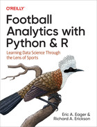
Base R contains useful diagnostic tools for looking at the results of linear models. The tools use base R’s plot() function (this is one of the few times we like plot(); it creates a simple function that we use only for internal diagnosis, not to share with others). First, use par(mfrow=c(2,2)) to create four subplots. Then plot() the multiple regression you previously fit and saved as expected_yards_r to create Figure 4-13:
## Rpar(mfrow=c(2,2))plot(expected_yards_r)
Figure 4-13 contains four subplots. The top left shows the model’s estimated (or fitted) values compared to the difference in predicted versus fitted (or residual). The top right shows cumulative distribution of the model’s fits against the theoretical values. The bottom left shows the fitted values versus the square root of the standardized residuals. The bottom right shows the influence of a parameter on the model’s fit against the standardized residual.

Figure 4-13. Four diagnostic subplots for a regression model
The “Residuals vs. Fitted” subplot does not look too pathological. This subplot simply shows that many data points do not fit the model well and that a skew exists with the data. The “Normal Q-Q” subplot shows that many data points start to diverge from the expected model. Thus, our model does not fit the data well in some cases. The “Scale-Location” subplot shows similar patterns as the “Residuals vs. Fitted.” Also, this plot has a weird pattern with W-like lines near 0 due to the integer (e.g., 0, 1, 2, 3) nature of the data. Lastly, “Residuals vs. Leverage” shows that some data observations have a great deal of “leverage” on the model’s estimates, but these fall within the expected range based on their Cook’s distance. Cook’s distance is, informally, the estimated influence of an observation on the model’s fit. Basically, a larger value implies that an observation has a greater effect on the model’s estimates.
Let’s look at what happens if you remove plays less than 15 yards or greater than 90 to create Figure 4-14:
## Rexpected_yards_filter_r<-pbp_r_run|>filter(rushing_yards>15&rushing_yards<90)|>lm(formula=rushing_yards~1+down+ydstogo+down:ydstogo+yardline_100+run_location+score_differential)par(mfrow=c(2,2))plot(expected_yards_filter_r)
Figure 4-14. This figure is a re-creation of Figure 4-13 with the model including only rushing plays with more than 15 yards and less than 95 yards
Figure 4-14 shows that the new linear model, expected_yards_filter_r, fits better. Although the “Residuals vs. Fitted” subplot has a wonky straight line (reflecting that the data has now been censored), the other subplots look better. The most improved subplot is “Normal Q-Q.” Figure 4-13 has a scale from –5 to 15, whereas this plot now has a scale from –1 to 5.
As one last check, look at the summary of the model and notice the improved model fit. The
## Rsummary(expected_yards_filter_r)
Which results in:
Call:
lm(formula = rushing_yards ~ 1 + down + ydstogo + down:ydstogo +
    yardline_100 + run_location + score_differential, data = filter(pbp_r_run,
    rushing_yards > 15 & rushing_yards < 95))


Residuals:
    Min      1Q  Median      3Q     Max
-17.158  -7.795  -3.766   3.111  63.471


Coefficients:
                    Estimate Std. Error t value Pr(>|t|)
(Intercept)        21.950963   2.157834  10.173   <2e-16 ***
down2              -2.853904   2.214676  -1.289   0.1976
down3              -0.696781   2.248905  -0.310   0.7567
down4               0.418564   3.195993   0.131   0.8958
ydstogo            -0.420525   0.204504  -2.056   0.0398 *
yardline_100        0.130255   0.009975  13.058   <2e-16 ***
run_locationmiddle  0.680770   0.562407   1.210   0.2262
run_locationright   0.635015   0.443208   1.433   0.1520
score_differential  0.048017   0.019098   2.514   0.0120 *
down2:ydstogo       0.207071   0.224956   0.920   0.3574
down3:ydstogo       0.165576   0.234271   0.707   0.4798
down4:ydstogo       0.860361   0.602634   1.428   0.1535
---
Signif. codes:  0 '***' 0.001 '**' 0.01 '*' 0.05 '.' 0.1 ' ' 1

Residual standard error: 12.32 on 3781 degrees of freedom
Multiple R-squared:  0.05074,   Adjusted R-squared:  0.04798
F-statistic: 18.37 on 11 and 3781 DF,  p-value: < 2.2e-16
In summary, looking at the model’s residuals helped you to see that the model does not do well for plays shorter than 15 yards or longer than 95 yards. Knowing and quantifying this limitation at least helps you to know what you do not know with your model.
Data Science Tools Used in This Chapter
This chapter covered the following topics:
-
Fitting a multiple regression in Python by using
OLS()or in R by usinglm() -
Understanding and reading the coefficients from a multiple regression
-
Reapplying data-wrangling tools you learned in previous chapters
-
Examining a regression’s fit
Exercises
-
Change the carries threshold from 50 carries to 100 carries. Do you still see the stability differences that you found in this chapter?
-
Use the full
nflfastRdataset to show that rushing is less efficient than passing, both using yards per play and EPA per play. Also inspect the variability of these two play types. -
Is rushing more valuable than passing in some situations (e.g., near the opposing team’s end zone)?
-
Inspect James Conner’s RYOE values for his career relative to Bell’s. What do you notice about the metric for both backs?
-
Repeat the processes within this chapter with receivers in the passing game. To do this, you have to filter by
play_type == "pass"andreceiver_idnot beingNAorNULL. Finding features will be difficult, but consider the process in this chapter for guidance. For example, usedownanddistance, but maybe also use something likeair_yardsin your model to try to set an expectation.
Suggested Readings
The books listed in “Suggested Readings” also apply for this chapter. Building upon this list, here are some other resources you may find helpful:
-
The Chicago Guide to Writing about Numbers, 2nd edition, by Jane E. Miller (Chicago Press, 2015) provides great examples for describing numbers in different forms of writing.
-
The Chicago Guide to Writing about Multivariate Analysis, 2nd edition, by Jane E. Miller (University of Chicago Press, 2013) provides many examples describing multiple regression. Although we disagree with her use of multivariate regression as a synonym for multiple regression, the book does a great job proving examples of describing regression outputs.
-
Practical Linear Algebra for Data Science by Mike X Cohen (O’Reilly Media, 2022) provides understanding of linear algebra that will help you better understand regression. Linear algebra forms the foundation of almost all statistical methods including multiple regression.
-
FiveThirtyEight contains a great deal of data journalism and was started and run by Nate Silver, until he exited from the ABC/Disney-owned site in 2023. Look through the posts and try to tell where the site uses regression models for posts.
-
Statistical Modeling, Causal Inference, and Social Science, created by Andrew Gelman with contributions from many other authors, is a blog that often discusses regression modeling. Gelman is a more academic political scientist version of Nate Silver.
-
Statistical Thinking by Frank Harrell is a blog that also commonly discusses regression analysis. Harrell is a more academic statistician version of Nate Silver who usually focuses more on statistics. However, many of his posts are often relevant to people doing any type of regression analysis.