CHAPTER 6
Messaging
Large-scale data-intensive applications need coordination between the parallel processes to achieve meaningful objectives. Since applications are deployed in many nodes within a cluster, messaging is the only way to achieve coordination while they execute.
It is fair to say that when large numbers of machines are used for an application, performance depends on how efficiently it can transfer messages among the distributed processes. Developing messaging libraries is a challenging task and requires years of software engineering to produce efficient, workable, and robust systems. For example, the Message Passing Interface (MPI) standard–based frameworks celebrated 25 years of development and are still undergoing retooling thanks to emerging hardware and applications.
There are many intricate details involved in programming with networking hardware, making it impossible for an application developer to fashion a program directly using hardware features. Multiple layers of software have been developed to facilitate messaging. Some of these layers are built into the operating system, with others at the firmware level and many at the software library level.
Nowadays, computer networks are operating continuously everywhere, transferring petabytes of data that touch every aspect of our lives. There are many types of networks that are designed to work in various settings, including cellular networks, home cable networks, undersea cables that carry data between continents, and networks inside data centers. Since data-intensive applications execute in clusters inside data centers, we will look at networking services and messaging within a data center.
Network Services
Computer networks are at the heart of distributed computing, facilitating data transfer on a global scale. This is a complex subject with rich hardware and software stacks. It is outside the scope of this book to go into details on networking. Instead, we will focus on those services offered by the networking layer to the application layer.
Popular networks used today offer applications the option of byte streaming services, messaging services, or remote memory management services. On top of this, other quality-of-service features such as reliable messaging and flow control are available. Applications can choose from these services and combine them with the required quality of service attributes to create efficient messaging services that are optimum for their needs.
Ethernet and InfiniBand are the two dominant networking technologies used in data centers. There are many other networking technologies available, though none is quite as popular due to price, availability of libraries, APIs, and the knowledge required to program them.
TCP/IP
Transport Control Protocol/Internet Protocol (TCP/IP) provides a stream-based reliable byte channel for communication between two parties. TCP/IP only considers bytes and how to transfer them reliably from one host to another and has a built-in flow control mechanism to slow down producers in case of network congestion.
TCP is programmed using a socket API. It has a notion of a connection and employs a protocol at the beginning to establish a virtual bidirectional channel between two parties looking to communicate. Once the connection is formed, bytes can be written to or read from the channel. Since there is no notion of a message in the TCP protocol, the application layer needs to define messaging protocols.
There are two popular APIs used for programming TCP applications using the socket API. They are blocking socket API and nonblocking socket API. With the blocking API, calls to write or read bytes will block until they complete. As a result we need to create threads for handling connections. If there are many simultaneously active connections, this method will not scale. With a nonblocking API, the read or write calls will return immediately without blocking. It can work in an event-driven fashion and can use different thread configurations to handle multiple connections. As such, most applications that deal with a significant number of connections use the nonblocking API.
Direct programming on the socket API is a laborious task owing to the specialized knowledge required. Popular programming languages and platforms used today have TCP libraries that are well recognized and used throughout applications. Data analytics applications depend on these libraries to transport their data messages.
RDMA
Remote direct memory access (RDMA) is a technique used by messaging systems to directly read from or write to a remote machine's memory. Direct memory access (DMA) is the technology used by devices to access the main memory without the involvement of the CPU.
There are many technologies and APIs that enable RDMA, providing low latencies in the nanosecond range and throughput well beyond 100Gbps. These characteristics have contributed to them being widely used in the high-performance and big data computing domains to scale applications up to thousands of nodes. Due to the high communication demands of distributed deep learning, they are employed in large deep learning clusters as well. RDMA technologies are available in the following forms:
- RDMA over Converged Ethernet (RoCE)—RoCE is a network protocol that allows remote memory access over an Ethernet network. It defines the protocol used over Ethernet.
- iWARP—This is a protocol defined on Internet Protocol networks such as TCP to provide RDMA capabilities.
- InfiniBand—Networking hardware that supports RDMA directly. InfiniBand networks are used in high-performance computing environments. They are found in data centers and big data clusters to accelerate processing.
InfiniBand networks can bypass the CPU and operating system (OS) kernel for packet processing, freeing valuable resources for computations. RDMA technologies use polling to figure out network events rather than interrupts to avoid the OS kernel. Apart from RDMA, InfiniBand networks support other messages such as send/receive, multicast, and remote atomic operations. All these features are used to build highly efficient messaging solutions within data centers.
Messaging for Data Analytics
Peer-to-peer messaging is the most basic form of transferring data between processes. Unless hardware features of networking fabrics are used, messages are always transferred between two processes. Even the most complex messaging patterns are created using peer-to-peer messaging primitives.
Anatomy of a Message
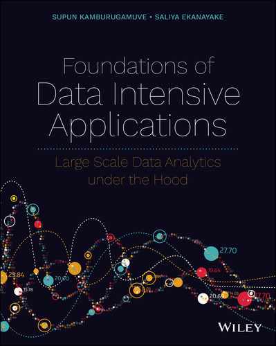
Now, let us examine some of the important steps we need to take to send a message from one computer to another. Assume we have an object we need to send to the other party. The object can be an array, a table, or something more complex such as a Java object. Figure 6-1 shows the steps taken by an application to send data to another computer.
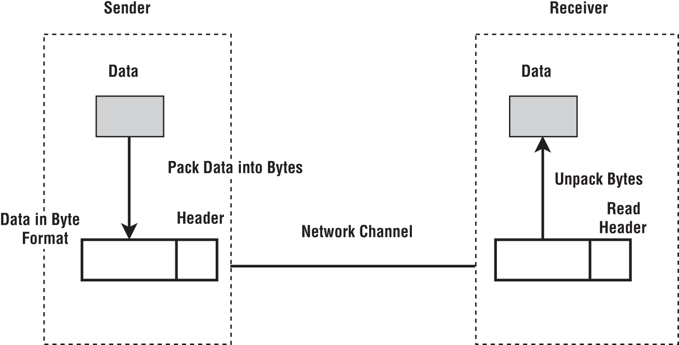
Figure 6-1: A message with a header. The header is sent through the network before the data.
Data Packing
First, we need to convert the data into binary format. We call this step data packing or serialization, and it depends on how we keep the data in the memory. In case our data is a C-style array, it is already in a contiguous byte buffer in the memory. If it is a table structure in a format like Apache Arrow, the data may be in multiple buffers each allocated for holding a data column of the table. In the case of Apache Arrow, there can be auxiliary arrays associated with the data arrays to hold information like null values and offsets. But the data is still in a set of contiguous buffers. In both a C-style array and an Arrow table, we can directly send the byte buffers without converting the original data structure.
If our data is in a more generic type such as a Java object, it is not in a contiguous buffer, and we may need to use an object serialization technology to convert it to a byte buffer. At the receiver, we need to unpack the data in the byte format and create the expected objects. To do this, we need information such as data types and the size of the message.
Protocol
A protocol is a contract between a sender and receiver so that they can successfully send messages and understand them. There are many messaging protocols available to suit our needs. Some are designed to work across hardware, operating systems, and programming languages. These protocols are based on open standards, with HTTP being familiar to most developers. Since such protocols are open, they sometimes present overheads for certain applications. For example, HTTP is a request-response protocol, but not every use case needs a response. The advantage of open protocols is that they allow various systems to be integrated in a transparent way.
Data-intensive frameworks tend to use internal protocols that are optimized for their use cases. The details of these protocols are not exposed to the user. Standard protocols are too expensive for the fine-grained operations occurring between the parallel processes of these frameworks.
There are two broad messaging protocols used for transferring data inside clusters. In the literature on messaging, they are called Eager Protocol and Rendezvous Protocol.
- Eager Protocol—The sender assumes there is enough memory at the receiving side for storing the messages it sends. When this assumption is made, we can send messages without synchronizing with the receiver. The Eager Protocol is more efficient at transferring small messages.
- Rendezvous Protocol—The sender first indicates to the receiver their intention to send a message. If the receiver has enough memory/processing to receive the message, it delivers an OK message back to the sender. Upon receiving this signal, the sender transmits the message. This protocol is mostly used for transferring larger messages.
The header contains the information needed by the receiver to process the message. Some common information in the header is listed here:
- Source identifier—Many sources may be sharing the same channel.
- Destination identifier—If there are many processing units at the receiver, we need an identifier to target them.
- Length—Length of the message. If the header supports variable-length information, we need to include its length.
- Data type—This helps the receiver to unpack the data.
As we can see, a header of a message can take up a substantial amount of space. If we specify the previous information as integers, the header will take up 16 bytes. If our messages are very small, we are using a considerable amount of bandwidth for the headers. After the receiver constructs the message, it can hand it over to the upper layers of the framework for further processing.
Message Types
A distributed data analytics application running in parallel needs messaging at various stages of its life cycle. These usages can be broadly categorized into control messages, external data source communications, and data transfer messages.
Control Messages
Data analytics frameworks use control messages for managing the applications in a distributed setting. The control messages are active in the initialization, monitoring, and teardown of the applications. Most are peer-to-peer messages, while some advanced systems have more complex forms to optimize for large-scale deployments. We touched upon control messages in an earlier chapter where we discussed resource management.
An example of a control message is a heartbeat used for detecting failures at parallel workers. In some distributed systems, parallel workers send a periodic message to indicate their active status to a central controller, and when these messages are missing, the central controller can determine whether a worker has failed.
External Data Sources
Data processing systems need to communicate with distributed storage and queuing systems to read and write data. This happens through the network as data are hosted in distributed data storages. Distributed storage such as file systems, object storages, SQL databases, and NoSQL databases provide their own client libraries so users can access data over the network. Apart from requiring the URL of these services, most APIs completely hide the networking aspect from the user.
We discussed accessing data storage in Chapter 2, so we will not go into more detail here. An example is accessing an HDFS file. In this case, the user is given a file system client to read or write a file in HDFS where the user does not even know whether that data is transferred through the network. In the HDFS case, the API provided is a file API. Databases offer either SQL interfaces or fluent APIs to access them. Message queues are a little different from other storage systems since they provide APIs that expose the messaging to the user. Reading and writing data to message queues is straightforward.
Data Transfer Messages
Once an application starts and data is read, the parallel workers need to communicate from time to time to synchronize their state. Let us take the popular big data example of counting words. To make things simple, we will be counting the total number of words instead of counting for individual words. Now, assume that we have a set of large text files stored in a distributed file system and only a few machines are available to perform this calculation.
Our first step would be to start a set of processes to do the computation. We can get the help of a resource manager as described in Chapter 3 and thereby manage a set of processes. Once we start these processes, they can read the text files in parallel. Each process will read a separate set of text files and count the number of words in them.
We will have to sum the word counts in different processes to get the overall total. We can use the network to send the counts to a single process, as shown in Figure 6-2. This can be achieved with a TCP library. First, we designate a process that is going to receive the counts. Then we establish a TCP connection to the designated receive process and send the counts as messages. Once the designated process receives messages from all other processes, it can calculate the total sums.

Figure 6-2: Processes 1, 2, and 3 send TCP messages to Process 0 with their local counts.
The previous example uses point-to-point messages, but collectively they are doing a summation of values distributed in a set of processes. A distributed framework can provide point-to-point messages as well as higher-level communication abstractions we call distributed operators.
- Point-to-point messages—This is the most basic form of messaging possible in distributed applications. The example we described earlier was implemented using point-to-point messages. These are found in programs that need fine-grained control over how parallel processes communicate.
- Distributed operations—Frameworks implement common communication patterns as distributed operations. In modern data-intensive frameworks, distributed operations play a vital role in performance and usability. They are sometimes called collective operations [1].
Most data-intensive frameworks do not provide point-to-point message abstractions between the parallel processes. Instead, they expose only distributed operations. Because of this, in the next few sections, we will focus our attention on distributed operations.
Distributed Operations
A distributed operation works on data residing in multiple computers. An example is the shuffle operation in map-reduce where we rearrange data distributed in a set of nodes. Distributed operations are present in any framework designed for analyzing data using multiple computers.
The goal of a distributed operation is to hide the details of the network layers and provide an API for common patterns of data synchronization. Underneath the API, it may be using various network technologies, communication protocols, and data packing technologies.
How Are They Used?
As discussed in Chapter 5, there are two methods of executing a parallel program: as a task graph or as a set of parallel processes programmed by the user. We can examine how distributed operations are applied in these settings. Irrespective of the setting, the operations achieve the same fundamental objectives.
Task Graph
Distributed operations can be embedded into a task graph–based program as a link between two tasks. Figure 6-3 details a computation expressed as a graph with a source task connected to a task receiving the reduced values through a Reduce link.

Figure 6-3: Dataflow graph with Source, Reduce Op, and Reduce Tasks (left); execution graph (right)
At runtime, this graph is transformed into one that executes on a distributed set of resources. Sources and reduced tasks are user-defined functions. The Reduce link between these nodes represents the distributed operation between them. The framework schedules the source and targets of the distributed operation in the resources according to the scheduling information. Figure 6-3 illustrates the transformed graph with four source task instances connected to a Reduce task instance by the Reduce distributed operation.
As we discussed in Chapter 5, the task graph–based execution is used in programs with a distributed data abstraction such as Apache Spark. The following Apache Spark example uses the Resilient Distributed Data (RDD) API to demonstrate a Reduce operation.
In this example, we have an array and partition it to 2 (parallelism). Then we do a Reduce operation on the data in the array. Note that Spark by default does the summation over all elements of the array and produces a single integer value as the sum. Spark can choose to run this program in two nodes of the cluster or in the same process depending on how we configure it. This API allows Spark to hide the distributed nature of the operation from the users.
import java.util.Arrays;import org.apache.spark.api.java.JavaRDD;import org.apache.spark.api.java.JavaSparkContext;public class SparkReduce {public static void main(String[] args) throws Exception {JavaSparkContext sc = new JavaSparkContext();// create a list and parallelize it to 2JavaRDD<Integer> list = sc.parallelize(Arrays.asList(4, 1, 3, 4, 5, 7, 7, 8, 9, 10), 2);// get the sumInteger sum = list.reduce((accum, n) -> (accum + n));System.out.println("Sum: " + sum);}}
Parallel Processes
As previously described, the MPI implementations provide distributed operations so that we can write our program as a set of parallel processes. Table 6-1 shows a popular implementation of the MPI standard [2]. The standard provides APIs for point-to-point communication as well as array-based distributed operations called collectives.
Table 6-1: Popular MPI Implementations
| MPI IMPLEMENTATION | DESCRIPTION |
|---|---|
| MPICH1 | One of the earliest MPI implementations. Actively developed and used in many supercomputers. |
| OpenMPI2 | Actively developed and widely used MPI implementation. The project started by merging three MPI implementations: FT-MPI from the University of Tennessee, LA-MPI from Los Alamos National Laboratory, and LAM/MPI from Indiana University. |
| MVAPICH3 | Also called MVAPICH2, developed by Ohio State University. |
With the default MPI model, the user programs a process instead of a dataflow graph. The distributed operations are programmed explicitly by the user between these processes in the data analytics application. Computations are carried out as if they are local computations identifying the parallelism of the program. This model is synonymous with the popular bulk synchronous parallel (BSP) programming model. In Figure 6-4, we see there are computation phases and distributed operations for synchronizing state among processes.

Figure 6-4: MPI process model for computing and communication
In the following source code, we have an
MPI_reduce
operation. Every parallel process generates a random integer array, and a single reduced array is produced at Process 0. The target is specified in the operation (in this case the 0th process), and the data type is set to Integer. Since the operation uses the
MPI_COMM_WORLD
, it will use all the parallel processes as sources. This API is a little more involved than the Spark version in terms of the parameters provided to the operation. Also, the semantics are different compared to Spark as the MPI program does an element-wise reduction of the arrays in multiple processes.
#include <stdio.h>#include <stdlib.h>#include <mpi.h>#include <assert.h>#include <time.h>int main(int argc, char** argv) {MPI_Init(NULL, NULL);int world_rank;MPI_Comm_rank(MPI_COMM_WORLD, &world_rank);int int_array[4];int i;printf("Process %d array: ", world_rank);for (i = 0; i < 4; i++) {int_array[i] = rand() % 100;printf("%d ", int_array[i]);}printf(" ");int reduced[4] = {0};// Reduce each value in array to process 0MPI_Reduce(&int_array, &reduced, 4, MPI_INT, MPI_SUM, 0, MPI_COMM_WORLD);// Print the resultif (world_rank == 0) {printf("Reduced array: ");for (i = 0; i < 4; i++) {printf("%d ", reduced[i]);}printf(" ");}MPI_Finalize();}
With MPI's parallel process management and the ability to communicate between them, we can build various models of distributed computing. We can even develop task graph–based executions using the functions provided by MPI [3]. Since MPI provides only the basic and most essential functions for parallel computing, its implementations are efficient. Even on large clusters, microsecond latencies are observed for distributed operations.
On the other hand, the simplistic nature of these functions creates a barrier for new users. Most MPI implementations lack enterprise features such as gathering statistics and web UIs, which in turn make them unattractive for mainstream users. With deep learning frameworks, MPI is increasingly used for training larger models and continues to gain momentum in data analytics.
Anatomy of a Distributed Operation
Now, let us look at the semantics of distributed operations and the requirements of the APIs.
Data Abstractions
The semantics of a distributor operation depend on the data abstractions and application domain they represent. As discussed in Chapter 4, arrays and tables are the two most common structures used in data-intensive applications.
- Arrays—We use arrays to represent mathematical structures such as vectors, matrices, and tensors. Distributed operations on arrays define the common communication patterns used in parallel calculations over these mathematical structures.
- Tables—The operations associated with tables originate from relational algebra. Distributed operations on tables include these relational algebra operations and common data transfer patterns such as shuffle.
Distributed Operation API
As distributed operations are built on messaging, they need the information we discussed for messaging and more to produce higher-level functionality.
Data Types
Arrays and tables are composite data structures. The actual data within these data types can be of distinct types such as Integers, Doubles, or Strings. Some distributed operations need access to this information. For example, to sort a table based on a string column, the operation needs to know that the column contains strings. Arrays are associated with a single data type. A table can have distinct data types in its columns, and we call this data type information a schema.
Sources and Targets
Assume a distributed operation is transpiring among N processes. Between these processes, there can be many entities producing and receiving data in the same operation. We call the entities producing the data to be source and those consuming the data are targets. Sources and targets can overlap, and in some cases they can even be the same. In general, sources and targets are logical entities and can be mapped to more concrete resources such as processes or threads.
Edge/Stream/Tag
Now, what would happen if we deployed two instances of the same operation at the same time? The receivers can receive messages without knowing exactly what operation to which they belong. An instance of an operation needs an identifier so that the messages between different instances running contemporaneously can be distinguished from one another. Some systems call this identifier a tag, while others refer to it as an edge or stream. Certain systems generate the identifier automatically without the user even being aware of its presence.
User Functions
Some distributed operations accept user-defined functions. These can specify operations on data or specify how to arrange the data in a distributed setting. For example, they can accept custom reduction functions and partitioning functions.
Streaming and Batch Operations
So far, we have looked at a distributed operation as taking input and producing output working across parallel processes. There is a difference in how the operations are used in batch and streaming systems. Streaming distributed operations accept input data continuously and produce outputs continuously. The batch operations use a finite amount of input data and at the end, produce an output by processing the data.
Streaming Operations
Streaming systems are always modeled as task graphs, and they run as long-running tasks and communication links. So, the streaming operations are running continuously, connecting the tasks by taking input from source tasks, and producing output to the receiving tasks.
Batch Operations
Two variants of batch operations are possible depending on whether the operations are designed to process in-memory data or large data.
- In-memory data—For in-memory data, an operation can take the complete data at once and produce the output. This simplifies the operation API. For example, array-based operations in MPI are designed around this idea.
- Large data—To handle large data that does not fit into the memory, the operation needs to take in data piece by piece and produce output the same way. The operation design is much more involved, as it needs to take partial input, process this using external storage, and take more input until it reaches the end. At the end, it still needs to produce output one chunk at a time.
Distributed Operations on Arrays
As we discussed in Chapter 4, arrays are one of the foundational structures for computing. They are used in machine learning, deep learning, and computer simulations extensively. When we have multiple arrays distributed over a cluster, we can apply array-based distributed operations. Table 6-2 shows some widely used examples on arrays.
Table 6-2: Common Distributed Operations on Arrays
| OPERATION | DESCRIPTION |
|---|---|
| Reduce, AllReduce | Elementwise reduction of array elements. |
| Gather, AllGather | Gathers multiple arrays together to form a larger array. |
| Broadcast | Sends a copy of an array to each target process. |
| Scatter | Partitions an array and sends those partitions to separate targets. |
| AllToAll | All the processes (sources) send data to all the other processes (targets). |
Distributed operations consider arrays as a sequence of elements (vectors) and apply operations accordingly. Note, that we can consider a single value as an array with one element. The following sections assume arrays are present in several processes. The semantics for the operations are based on the MPI standard.
Broadcast
Broadcast is widely used by programs to send a copy of data to multiple processes from a single process. Broadcast is easy to understand and can be found in all major systems designed to process data in parallel. Figure 6-5 has five parallel processes with IDs assigned from 0 to 4. The 0th process has an array it must broadcast to the rest; at the end of the operation, all the processes will have a copy of this array.
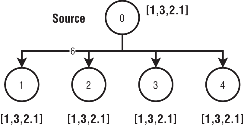
Figure 6-5: Broadcast operation
Broadcast does not consider the structure of the array, meaning it can be anything, such as a byte array created from a serialized object.
Reduce and AllReduce
Reduce is a popular operation for computations on arrays. A reduction is associated with a function, and the following are some popular examples:
- Sum
- Multiply
- Max
- Min
- Logical or
- Logical and
Commutativity is a key factor when considering Reduce functions. All those listed here are commutative functions. An example of a noncommutative function is division. A binary operator ![]() is commutative if it satisfies the following condition:
is commutative if it satisfies the following condition:
If a reduction function is commutative, the order of how it is applied to data does not matter. But if it is noncommutative, the order of the reduction is important.
Now, let us look at the semantics of reductions on arrays. Each distributed process has the same size array. The values in every position of the array are reduced individually with the corresponding values from other arrays. The result is an array of the same size and data type. Here are four arrays:
- A = [10, 12]
- B = [20, 2]
- C = [40, 6]
- D = [10, 10]
The Reduce result for a sum function of these arrays is another array, R = [80, 30]. In Figure 6-6, the arrays are placed in tasks with IDs from 0 to 4. The Reduce result is given to Task 1.
AllReduce is semantically equivalent to Reduce followed by Broadcast, meaning reduced values are transferred to all the targets of the operation. This raises the question: why have a separate operation called AllReduce if Reduce and Broadcast already exist in the first place? First, this is a heavily used operation in parallel programs. As such, it deserves its own place since it would be unreasonable to expect users to use two operations for one of the most popular capabilities parallel programs require. Second, we can implement AllReduce in ways that are more efficient than Reduce followed by Broadcast implementations. Figure 6-7 shows the same example with AllReduce instead of Reduce. Now, the reduced value is distributed to all the tasks.
Figure 6-6: Reduce operation

Figure 6-7: AllReduce operation
Gather and AllGather
As the name suggests, the Gather operation takes values from multiple locations and groups them together to form a large set. When creating the set, implementations can preserve the source that produced the data or not, depending on preference. In classic parallel computing, the values are ordered according to the process identification number. Figure 6-8 shows a gather operation.
Similar to AllReduce, the AllGather operation is equivalent to combining Gather followed by Broadcast. It is implemented as a separate operation owing to its importance and the implementation optimizations possible. Figure 6-9 shows an AllGather example.

Figure 6-8: Gather operation

Figure 6-9: AllGather operation
Scatter
Scatter is the opposite of the Gather operation, as it distributes the values in a single process to many processes according to a criterion specified by the user. Figure 6-10 shows the scatter operation from Process 0 to four other processes.

Figure 6-10: Scatter operation
In the preceding Scatter operation, the first two consecutive values are sent to the first target, while the second set of consecutive values go to the second target.
AllToAll
AllToAll can be described as every process performing a scatter operation to all the other processes at the same time. Figure 6-11 has four arrays in four processes, each with four elements. The 0th element of these arrays goes to 0th process, and the 1st element of these arrays goes to 1st process. Once we rearrange the arrays like this, four new arrays are created in the four processes.
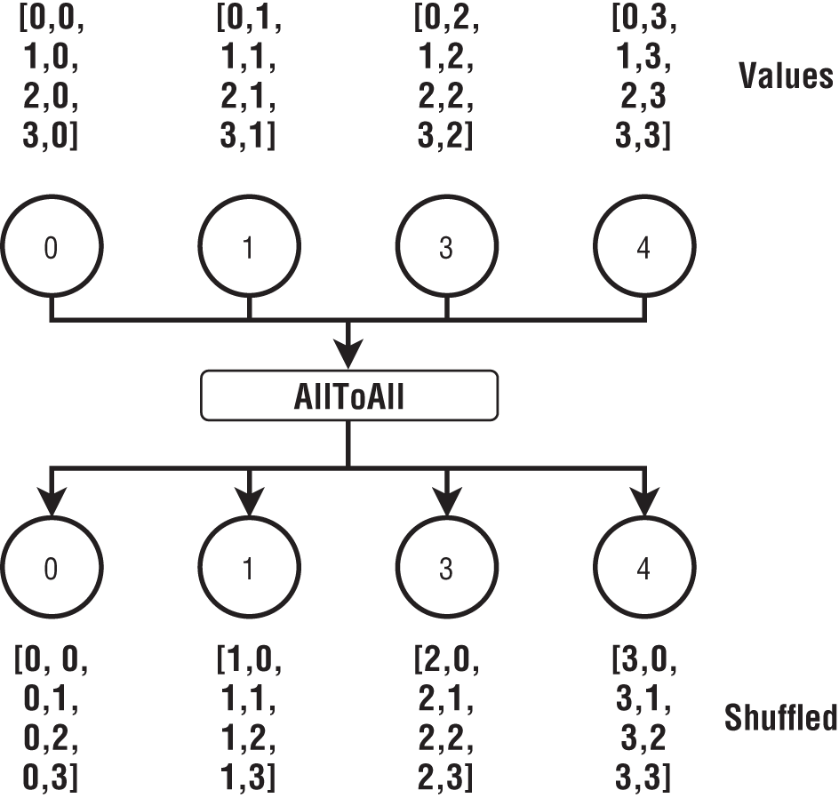
Figure 6-11: AllToAll operation
Optimized Operations
Messaging for parallel applications offers many challenges, especially when working in large, distributed environments. Much research has been devoted to improving these operations, with billions of dollars of research funding going toward enhancing the messaging libraries and network hardware for large-scale computations.
Let us take the previous example of summing up a set of values distributed over several processes. The approach we described before was to send the values from all processes to a single process. This is effective for small messages with a correspondingly small number of parallel processes. Now, imagine we need to send 1MB of data from 1,000 parallel processes. That single process needs to receive gigabytes of data, which can take about 1 second with a 10Gbps Ethernet connection with a theoretical throughput. After receiving 1GB of this data, the process must go through and add them as well.
When 1,000 processes try to send 1MB messages to a single process, the network becomes congested and drastically slows down, such that it can take several seconds for all the messages to be delivered. This can lead to network congestion and large sequential computations for a single process. In the 1980s, computer scientists realized they could use different routing algorithms for sending messages to avoid these problems. Such algorithms are now called collective algorithms and are widely used in optimizing [4] these distributed operations.
Broadcast
The simplest approach to implement Broadcast is to create N connections to the target processes and send the value through. In this model, if it takes ![]() time to put the Broadcast value into the network link, it will take
time to put the Broadcast value into the network link, it will take ![]() times to completely send the value to all N processes. Figure 6-12 illustrates this approach. It is termed a flat tree as it forms a tree with the source at the root and all the other workers at the leaves. This method works better if N is small and takes much longer when either N or the message size increases.
times to completely send the value to all N processes. Figure 6-12 illustrates this approach. It is termed a flat tree as it forms a tree with the source at the root and all the other workers at the leaves. This method works better if N is small and takes much longer when either N or the message size increases.
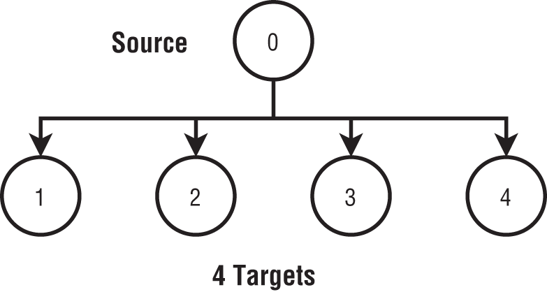
Figure 6-12: Broadcast with a flat tree
There are methods that can perform much better for many processes. One such option is to arrange the processes in a binary tree, as shown in Figure 6-13, and send the values through the tree. The source sends the value to two targets; these in turn simultaneously send the value to four targets, which transfer the value to eight targets, and so on until it reaches all targets. The parallelism of the operation increases exponentially, and as it expands, it uses more of the total available bandwidth of the network. Theoretically, it takes about ![]() steps to broadcast the values to all the nodes. When N is large, this can reduce the time required significantly.
steps to broadcast the values to all the nodes. When N is large, this can reduce the time required significantly.
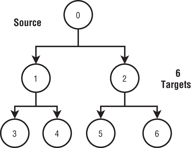
Figure 6-13: Broadcast with a binary tree
The tree approach works well only for smaller values that do not utilize the network fully. In the case of large messages, there is still a bottleneck in this approach since every node other than the leaves tries to send the value to two processes at the same time. The operation can be further optimized for larger data by using methods such as chaining and double trees. It is important to note that some computer networks have built-in capabilities to broadcast values, and implementations sometimes exploit these features.
Reduce
Depending on the message sizes, different routing algorithms can be utilized to optimize the performance of the Reduce operation. For smaller values, routing based on tree structures is optimal. The tree-based routing algorithms work by arranging the participating processes in an inverted tree. The root of the tree is the target that receives the final reduced value, and the rest of the tree are the sources producing the data to be reduced. As in the broadcast case, the reduction can be done in log N steps for N parallel processes.
AllReduce
The simplest form of AllReduce implementation is a Reduce operation followed by a Broadcast. This works well for small messages. When the message size is large, however, the network is not fully utilized. To optimize the network bandwidth utilization, a ring-based routing algorithm or recursive doubling algorithm can be used.
Ring Algorithm
In this version, data from each process is sent around a virtual ring created by the ith process connecting to the ![]() where
where ![]() is the number of processes. In the first step, each process sends its data to its connected process. In the next step, each process sends the data it received in the previous step to its connected process. This is done for
is the number of processes. In the first step, each process sends its data to its connected process. In the next step, each process sends the data it received in the previous step to its connected process. This is done for ![]() steps. The algorithm fully utilizes the available network bandwidth by activating all the network links equally at every step. It is best suited for large data reductions. Figure 6-14 shows a reduced set of values in four processes in three steps.
steps. The algorithm fully utilizes the available network bandwidth by activating all the network links equally at every step. It is best suited for large data reductions. Figure 6-14 shows a reduced set of values in four processes in three steps.
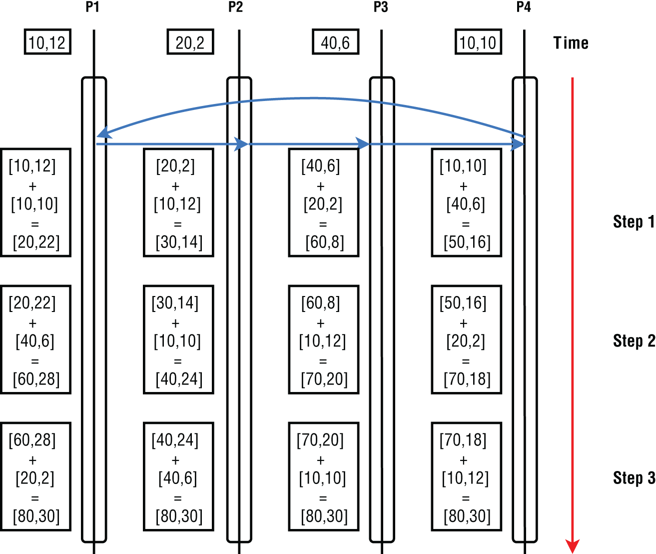
Figure 6-14: AllReduce with Ring
Recursive Doubling
Figure 6-15 shows the recursive doubling algorithm. Each process will start by sending data to a process at distance 1. For example, process 0 will send data to process 1. At each step ![]() , this distance will double until
, this distance will double until ![]() steps are completed. This algorithm takes
steps are completed. This algorithm takes ![]() steps to communicate the data between the processes. Figure 6-15 demonstrates how this algorithm works for four processes. The algorithm has better latency characteristics than the previous one but does not utilize the network as efficiently.
steps to communicate the data between the processes. Figure 6-15 demonstrates how this algorithm works for four processes. The algorithm has better latency characteristics than the previous one but does not utilize the network as efficiently.

Figure 6-15: AllReduce with recursive doubling
Gather and AllGather Collective Algorithms
Gather collective algorithms are inverted versions of the Broadcast algorithms. We can use flat trees or binary trees for small message sizes. Gather produces a large dataset when data size in individual processes or the number of parallel processes increases. Chaining algorithms are available for larger messages.
For AllGather operations, Gather followed by Broadcast is a viable option for small messages with a small number of processes. AllGather can transfer larger messages as it needs to distribute the gathered value to all the other processes. For these cases, one can use the ring algorithm or the recursive doubling algorithm described in the AllReduce.
Scatter and AllToAll Collective Algorithms
Scatter utilizes collective algorithms found in Broadcast for sending the values present in a single process to multiple processes. AllToAll can involve many communications as a result of sending data from each process to all the other processes. It can be optimized using a chaining algorithm. This algorithm works by arranging the processes in a dynamic chain configuration. At the kth step, the process ![]() sends data to the
sends data to the ![]() where
where ![]() is the number of processes. We will discuss this algorithm later along with shuffle.
is the number of processes. We will discuss this algorithm later along with shuffle.
Distributed Operations on Tables
As mentioned, data management systems are built around table abstractions. Whether Pandas DataFrame or Spark RDD, the processing semantics associated with them are similar because they have the same goal of representing data as a table. The operations in these systems are based on relational algebra [5] and SQL. Shuffle is the most widely used operation for implementing many of the relational algebra operations in a distributed setting. Table 6-3 lists some of the widely used operations we discussed in the previous chapter.
Table 6-3: Distributed Operations for Tables
| OPERATION | DESCRIPTION |
|---|---|
| Shuffle | Partition the tables and redistribute them. |
| Joins | Distributed joins using join, left outer join, right outer join, and full outer join. |
| GroupBy | Group the rows according to a key. |
| Aggregate | Aggregate functions such as SUM, MIN, MAX, AVG. |
| Sort | Sorting of tables based on columns. |
| Union | Union of two tables. |
| Difference | Set difference of two tables. |
| Broadcast | Broadcast a table to workers. |
Like with array based distributed operations, we have tables in a distributed setting. These can be partitions of a larger table depending on how our program models computations. For this discussion, we assume horizontal partitioning by rows. In the next few sections, we will look at how these operations are implemented.
Shuffle
The shuffle operation is designed to rearrange table data among a distributed set of workers. Shuffle is like AllToAll operation for arrays and works on tables instead. Since shuffle has AllToAll semantics, each node is potentially distributing data to all the other participating nodes.
Figure 6-16 demonstrates the major steps of shuffle. We have a table with two columns and four partitions distributed in a cluster. We are going to apply a shuffle operation to this data using the key as column K. After the shuffle, records with Key 1 will create Partition 0, records with Key 2 will create Partition 1, and so on.
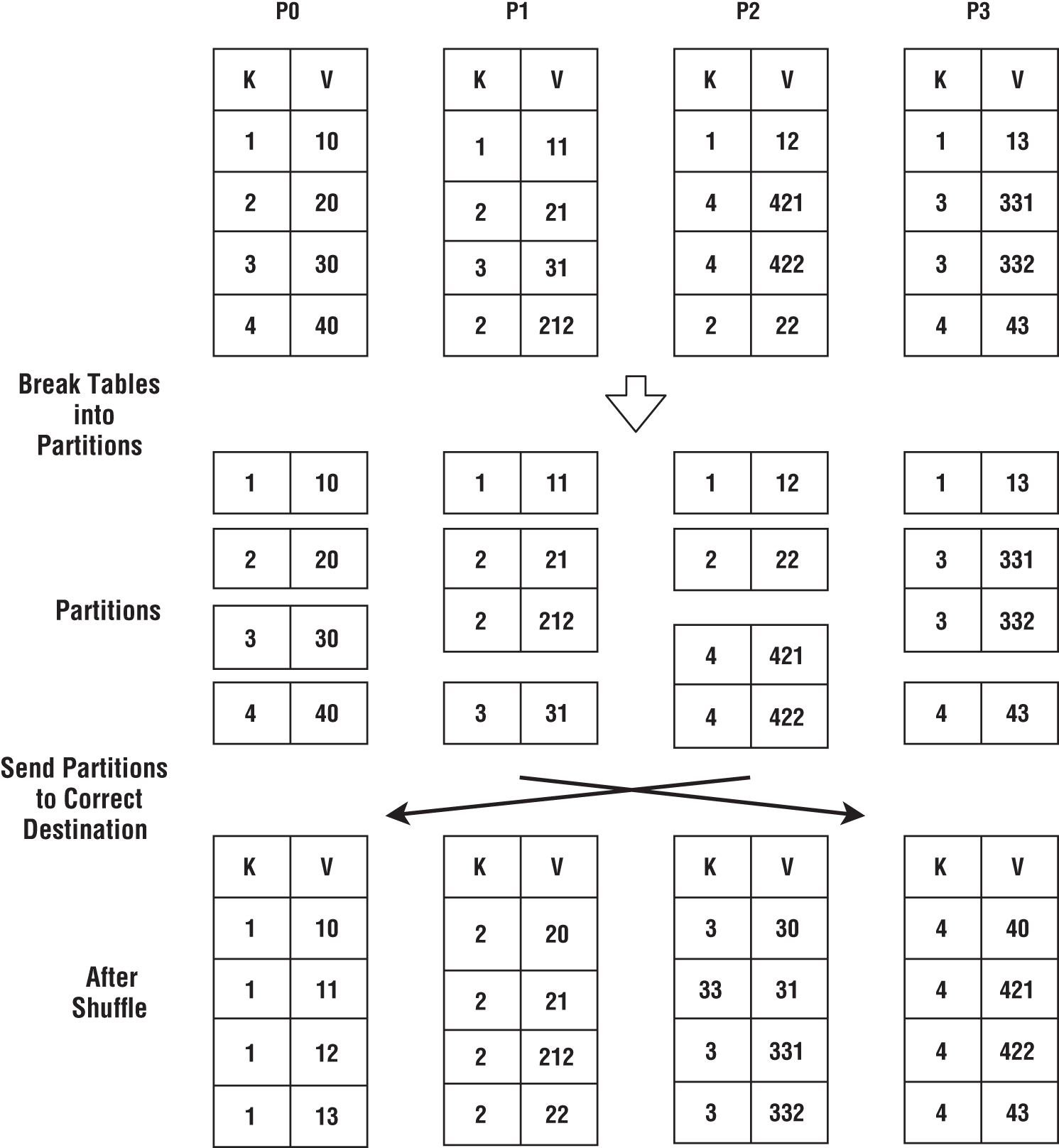
Figure 6-16: Shuffle operation
The shuffle operation is given the original tables. The first step it must take is to create local partitions according to the key, as shown in Figure 6-16. These partitions are then sent to the correct destinations. A receiver will get many partitions from different processes and combine them to create the final table.
Systems can use different algorithms to create the partitions and send them to the correct destinations.
Partitioning Data
For larger datasets, partitioning can take a considerable amount of time. The common partitioning schemes used in data-intensive frameworks are hash partitioning and radix partitioning.
Hash Partitioning
Assume we are going to create ![]() partitions from a dataset, and these are numbered from
partitions from a dataset, and these are numbered from ![]() to
to ![]() . We can apply a hashing function to the attribute value we are using to partition the data. The new partition
. We can apply a hashing function to the attribute value we are using to partition the data. The new partition ![]() of a record with attribute value
of a record with attribute value ![]() can be calculated by the following:
can be calculated by the following:
This operation can be time-consuming when large numbers of records need to be processed. If we have multiple attributes, we can use those values in the hash function. A hash function such as murmur or modulo [6] can perform the hashing.
Radix Partitioning
Radix partitioning [7] is a widely used technique in databases. It starts by creating a histogram of ![]() buckets using a radix of size
buckets using a radix of size ![]() . For example, if the radix is 10, it will create
. For example, if the radix is 10, it will create ![]() buckets. Then it goes through the data and counts the number of items for each bucket. This is done using
buckets. Then it goes through the data and counts the number of items for each bucket. This is done using ![]() bits of each attribute value. Here is a code snippet for calculating histogram for a 32-bit integer value:
bits of each attribute value. Here is a code snippet for calculating histogram for a 32-bit integer value:
histogram[input >> (32 - N)]++Now, using this histogram, we can calculate boundaries for ![]() partitions where
partitions where ![]() . We then go through the data again and assign them to the correct partitions.
. We then go through the data again and assign them to the correct partitions.
In a distributed setting, we need to calculate a global histogram from all the partitions. We can calculate a histogram for each partition and combine them using a Reduce operation to create the global histogram.
Load Balancing
When we shuffle the data, the resulting partitions assigned to a CPU core can be skewed. Imagine in our previous example we chose the partitioning scheme as Keys 1 and 2 going to the 0th partition, Key 3 going to the 2nd partition, and Key 4 going to the 3rd partition. Now data in the 1st partition is empty, while the 0th partition has twice the data as 2nd and 3rd partitions. This was a hypothetical example, but this scenario is common in practice, so choosing the correct partitioning method is important.
Depending on the number of buckets and the data distribution, radix can create an imbalanced partitioning. It is possible to increase the number of buckets in the histogram to reduce the load imbalance, but we may need more memory to create the histogram. A simple hash partitioning produces imbalanced partitions in numerous practical use cases. Depending on the data, we may need to use a custom partitioning method to make sure the resulting partitions are balanced.
Handling Large Data
Handling data larger than memory means we cannot keep all the data at once in memory. Therefore, we need to design the shuffle operation to take a stream of inputs to handle data larger than memory. Also, its output should be streamed out piece by piece. Since we are taking a stream of inputs, we can keep only part of the data in the memory at any instant.
To keep the parts that are not in memory, shuffle operation needs to tap into disk storage. Disks are orders of magnitude slower than the main memory and cheaper per storage unit by comparison.
The code works by reading a part of the data into memory and inserting that into the shuffle operation, as shown in Figure 6-17. The shuffle operation creates partitions and send them to the correct destinations. Once the receivers have these partitions, they can write them to disk so that they have enough memory to handle the next batch. Then we read the proceeding partitions from the disk and repeat the same until all the data are read from the disk.
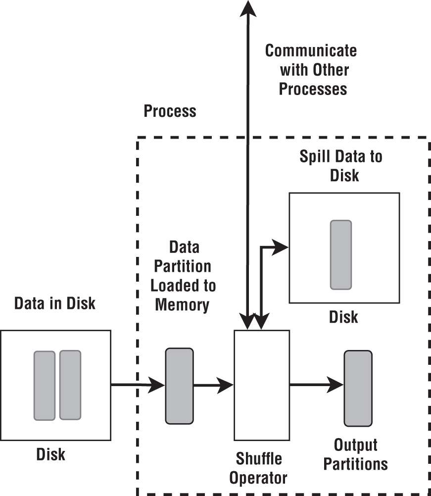
Figure 6-17: Shuffle with data that does not fit into memory
At this point, the operation can start outputting data in a streaming fashion one partition at a time. Shuffle has an option to sort records based on a key associated with that record. When sorting is enabled, an external sorting algorithm can be used. For example, at the receiver we can save data to the disk after sorting. When reading, we merge the sorted partition data.
Next, we will look at a few algorithms for implementing shuffle operation.
Fetch-Based Algorithm (Asynchronous Algorithm)
The fetch-based algorithm is a popular approach adopted by current big data systems that adopts asynchronous execution. We will discuss it in Chapter 7. Figure 6-18 illustrates how the input data to the operation is split into buffers. When the buffer becomes full, the data is spilled to the disk. To achieve maximum performance from a disk, read and write needs to be done with larger chunks and on contiguous regions.
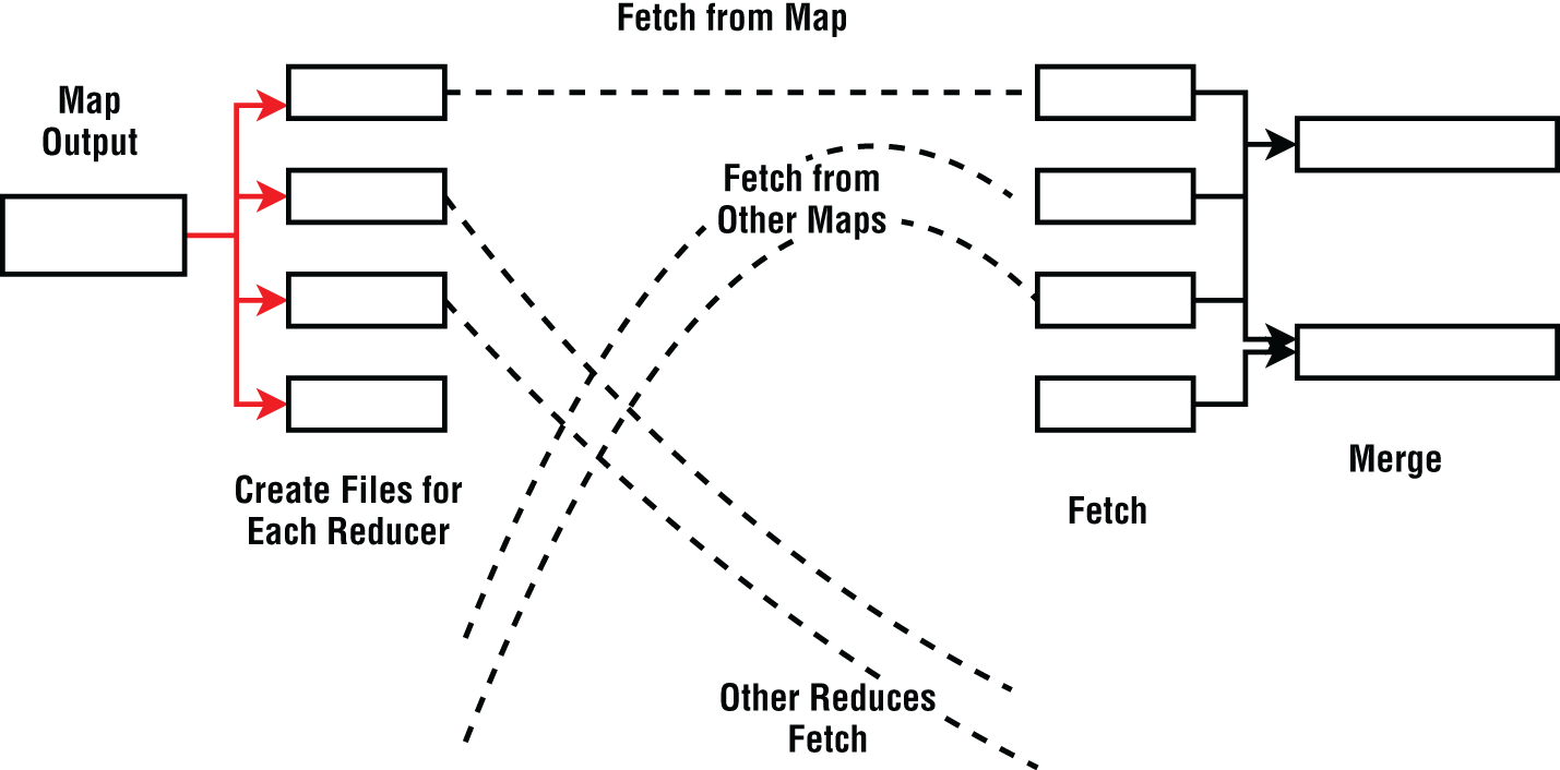
Figure 6-18: Fetch-based shuffle
The sources update a central server with the data location of partitions, and the targets get to know about the data to receive from this server. Bear in mind central synchronization does hold the risk of introducing potential performance bottlenecks when there are many parallel workers trying to synchronize all at once. After the target fetches data from multiple sources, they merge them utilizing the disk.
Distributed Synchronization Algorithm
The shuffle can be implemented as a distributed synchronization algorithm without a single point for coordination, as shown in Figure 6-19. This algorithm works by arranging the tasks in a chain configuration. The algorithm is self-synchronizing and can be used in high-performance clusters.
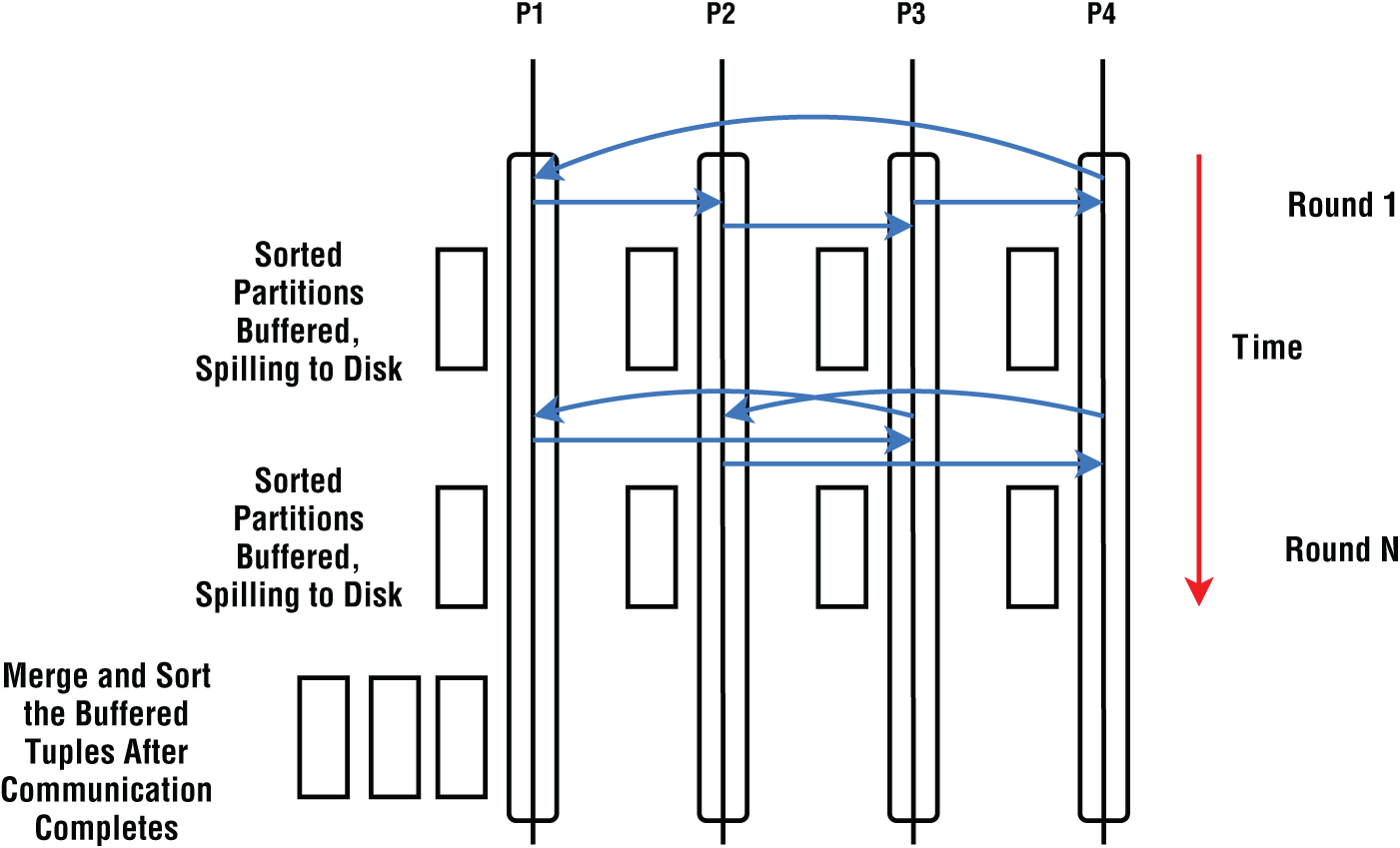
Figure 6-19: Chaining shuffle with four processes
The advantage of this is that it does not have the problem of overloading a single node with multiple senders transmitting to the same location. Also, it can utilize all the networking links fully without trying to send the messages through the same networking link at any given time. Unfortunately, it requires every node to participate in communication in synchronization with each other. If one node becomes slow, it can affect the whole algorithm. Such slowdowns can be due to factors such as garbage collection, network congestion, and operating system noise.
Shuffle deals with substantial amounts of data over phases of computation, communication, and disk I/O. By overlapping these phases, resources can be utilized to the fullest and improve the throughput. Most implementations found in big data systems support such overlapping to various degrees.
GroupBy
GroupBy followed by an aggregation operation is a popular method in big data systems. The original map-reduce paradigm was a GroupBy operation where a set of data in the form of a table (key, value) is shuffled and then grouped according to the key. It applies a Reduce (aggregate) operation to the values of the same key.
Figure 6-20 demonstrates the GroupBy operation with a summation aggregation. First, we shuffle the tables so that the same key goes to the same process. Then we do a local aggregation on the values of that key.

Figure 6-20: GroupBy operation
Aggregate
We looked at Reduce operations for arrays earlier. Aggregate operations in tables are like Reduce operations in arrays but with slightly different semantics. Aggregate operations are applied to a column of a table.
Let us take the example of a summation aggregate function. When applied to a column, the summation function adds up values of that column. When applied to a table distributed over a cluster, the aggregate function computes a global sum of the column values. In contrast, an array-based reduction adds up values in the same array indexes.
Figure 6-21 shows a SUM aggregate function on column V of the table distributed over two processes. We calculate the local sum for each process and then do a global sum using a reduce operation that works with arrays (array with one element).
![Schematic illustration of aggregate function sum on a distributed table [c06f021.png].](https://imgdetail.ebookreading.net/202111/01/9781119713029/9781119713029__9781119713029__files__images__c06f021.png)
Figure 6-21: Aggregate function sum on a distributed table
Join
Joins are time-consuming when large datasets are involved. A join requires two input datasets and outputs a single dataset. There are several types of joins available in data management systems:
- Inner join
- Left outer join
- Right outer join
- Full outer join
With the help of an example, let us look at the semantics of these operations. Here are two datasets we are going to use for the joins shown in a table format. Each dataset has a common attribute called Customer ID.
Data Set A (Customer details)
| CUSTOMER ID | NAME | PHONE | |
| 1 | John Doe | [email protected] | 891-234-9245 |
| 2 | Smith Rosenberry | [email protected] | 934-234-2321 |
| 3 | Jack Igor | [email protected] | 421-234-1234 |
| 4 | Ana Kelse | [email protected] | 233-123-4423 |
Data Set B (Orders)
| ORDER ID | CUSTOMER ID | ORDER DATE |
| 103 | 1 | 2020-02-10 |
| 223 | 3 | 2020-02-21 |
| 321 | 4 | 2020-02-11 |
Inner Join (Join)
An inner join creates a dataset with records that have matching values in both input datasets. Inner joins with equal conditions are one of the most often used in practice. Joins with equal conditions are called equijoins. Inner joins are referred to simply as joins. To find the relevant information of those customers who have an order, let us look at the output dataset for joining A and B with an equijoin using Customer ID as the key. The following table shows the results of this inner join:
| CUSTOMER ID | NAME | PHONE | ORDER ID | ORDER DATE | |
| 1 | John Doe | [email protected] | 891-234-9245 | 103 | 2020-02-10 |
| 3 | Jack Igor | [email protected] | 421-234-1234 | 223 | 2020-02-21 |
| 4 | Ana Kelsey | [email protected] | 233-123-4423 | 321 | 2020-02-11 |
Left (Outer) Join
Left join outputs the left dataset completely while taking the records from the right dataset where the join condition is met. For records from a left dataset without matching records from the right dataset, the right table fields are filled with NULL values.
Still using the current example, we are going to select all the customers and any order they might have. Note that the customer with Customer ID 2 does not have any orders, so their corresponding columns are set to NULL.
| CUSTOMER ID | NAME | PHONE | ORDER ID | ORDER DATE | |
| 1 | John Doe | [email protected] | 891-234-9245 | 103 | 2020-02-10 |
| 2 | Smith Rosenberry | [email protected] | 934-234-2321 | NULL | NULL |
| 3 | Jack Igor | [email protected] | 421-234-1234 | 223 | 2020-02-21 |
| 4 | Ana Kelsey | [email protected] | 233-123-4423 | 321 | 2020-02-11 |
Right (Outer) Join
Right join is the mirror of the left join, with all the records from the right dataset in the output. If the left join example's datasets are exchanged (the right dataset becomes the left, and the left dataset becomes the right) and applied to the right join with the same condition, it would produce the same results.
Full (Outer) Join
A full join produces a dataset by combining the results of both left and right outer joins and returns all rows irrespective of a match from the datasets on both sides of the join.
Dataset A
| A | B |
| 1 | x |
| 2 | y |
| 5 | z |
Dataset B
| A | C |
| 1 | p |
| 2 | q |
| 4 | r |
Here is a simple example of joining Dataset A and B on attribute A (equality) using a full join. There are two rows that match, and they share attributes for all. For nonmatching rows, the row from one table is given with missing values from the other table.
| A | B | C |
| 1 | x | p |
| 2 | y | q |
| 5 | z | NULL |
| 4 | NULL | r |
Join Algorithms
In most databases, the join algorithm occurs in a single machine, whereas with big data systems the joins take place in a distributed setting at a much larger scale. It is important to understand the mechanics of a join in a single machine to apply it on a larger scale. Hash join and sorted merge join algorithms are the most popular. Many frameworks implement both as they can be efficient for several types of joins with varying parameters. Depending on the situation, the correct join can be selected by the framework or the user.
Hash Join
Hash joins work by creating an in-memory hash map from one dataset. The algorithm has two phases:
- Hashing phase—Creates a hash map using one of the datasets. The key of the hash map is the join attribute, and the value is the actual record. The hash map should support a super-efficient lookup of values by way of the key. Usually this can be an
 lookup. The smaller relation is used for building the hash map.
 - Joining phase—After the hash map is created, the other table can be scanned and matched against the hash table. If a value is found in the hash table, these are then joined. Since the hash and equality are used for looking up the key, this method can only support joins with equal conditions.
We usually choose the smaller relationship to create the hash map.
Sorted Merge Join
The naive approach to joining two datasets is to take one record from a dataset and compare it against the entire next relationship to find if there are records matching the join condition. The pseudocode for this is shown in the following with datasets A and B:
For a in AFor b in BIf a and b matches join conditionAdd to output a,b
This approach needs a ![]() comparison, which can become huge as the size of the datasets increases. Imagine joining a million tuples against another million tuples. The previous algorithm requires 1,000 billion comparisons to complete. To avoid that many comparisons, the datasets can be sorted using the joining keys. The sorting can be done in
comparison, which can become huge as the size of the datasets increases. Imagine joining a million tuples against another million tuples. The previous algorithm requires 1,000 billion comparisons to complete. To avoid that many comparisons, the datasets can be sorted using the joining keys. The sorting can be done in ![]() time, and after this one scan through both datasets, it can join them together. If the number of records in relation A is N and the number of records in relation B is M, the complexity will be
time, and after this one scan through both datasets, it can join them together. If the number of records in relation A is N and the number of records in relation B is M, the complexity will be ![]() .
.
The algorithm is shown next and can be described in just a few steps. Initially, both datasets are sorted with the join key. Note that this algorithm works only for equijoins. The algorithm defines a function called
advance
that scans a given dataset starting with a given index. This function outputs the records with a key equivalent to the starting index of the scan. Since the datasets are sorted, it only needs to look at the consecutive elements. The moment it sees anything different, it can return the current set.
function sortMergeJoin(dataset L, dataset R, key k)dataset output = {}// sort L and R with key klist lSorted = sort(L, k)list rSorted = sort(R, k)key lKey, rKeyset lSubset, rSubsetadvance(lSubset, lSorted, lKey, k)advance(rSubset, rSorted, rKey, k)while not empty(lSubset) and not empty(rightSubset)if lKey == rKeyadd cartesian product of lSubset and rSubset to outputadvance(lSubset, lSorted, lKey, k)advance(rSubset, rSorted, rKey, k)else if left_key < right_keyadvance(lSubset, lSorted, lKey, k)elseadvance(rSubset, rSorted, rKey, k)return outputfunction advance(subset out, sortedData inout, key out, k in)key = sortedData[0].key(k)subset = {}while not empty(sortedData) and sortedData[0].key(k) == keysubset.insert(sorted[0])sortedData.remove(0)
After the
advance
function finds records for each dataset, if the keys are equal, the Cartesian product is taken of the two outputs of the advance, and then the
advance
function is run on both datasets. If the keys of a dataset are less than the other dataset, the algorithm runs the
advance
routine on the dataset with the lesser key starting from the previous end index. This assumes an ascending order sorting of the relationships. The algorithm does this until it reaches the end of one dataset. Figure 6-22 shows two relationships with two fields per record. The first field is taken as the joining key.

Figure 6-22: Sorted merge join
The output of the equijoin will be as follows:
[3,5,1], [3,5,2], [3,5,3], [3,6,1], [3,6,2], [3,6,3], [5,1,1], [5,0,1], [8,0,1], [8,9,1].
Notice how it takes the Cartesian product of the matching records of the two datasets. This algorithm works much more efficiently compared to two sets done naively for larger datasets. Sorting an enormous number of records can take a significant amount of time. When data larger than memory is involved, an external sorting algorithm is of great help.
Distributed Joins
The idea behind the distributed join is simple. It first redistributes data with the same keys from both datasets into the same processes. After this, the data in each process is joined separately using one of the join algorithms mentioned earlier [8]. Figure 6-23 shows an example of such where Process 0 and Process 1 has two tables 0 and 1. Process 0 has the 0th partition of these tables, and Process 1 has the 1st partition. First the data is shuffled so that Keys 1 and 2 go to Process 0 and Keys 3 and 4 are sent to Process 1. After the shuffle, the tables are joined locally.

Figure 6-23: Distributed join on two tables distributed in two processes
Performance of Joins
We described the basic structure of a join here, and in practice they are implemented to efficiently use the cache and reduce the TLB misses. First, the tables are partitioned into small datasets. This is done so that individual partitions fit into the cache to make sorting or hashing efficient.
A join can produce a dataset that is many times bigger than the input datasets. In classic implementations, the hash join is slightly better than the sort-merge join. Sort-merge join is a more popular implementation as it can handle all the join scenarios. The performance of these two algorithms depends on the implementation and programming environment.
The performance evaluations of the algorithms found in research literature are done mostly in ideal conditions. In practice, factors such as data representation in the memory and size of the data and whether disks are used can determine which implementation is faster. With such a complex set of circumstances, it is better to consult the performance numbers of specific frameworks and their recommendations to figure out the correct algorithm for certain situations.
There are many other optimizations available as well. For example, if one relationship is comparatively small, instead of reshuffling both tables, we can send the small table to all the processes and do the join at each process. This avoids the shuffling of the larger table that can take a considerable time.
More Operations
Table 6.4 shows a few other operations and how they are implemented in a distributed setting. All the operations in the table use shuffle, and some use a few other communication operations as well.
Table 6.4: Table-Based Operations and Their Implementations
| OPERATION | DESCRIPTION | IMPLEMENTATION |
|---|---|---|
| Union | Set union with duplicate removal. | Shuffle based on hash and local union. |
| Sort | Sorting values so there is a global ordering. For example, 0th process gets the lowest sorted values, 1st process gets the next sorted values, and so on. | Do sampling to determine the global partition boundaries. Requires a Gather operation and a broadcast for determining the partitioning using sampling. Then do shuffle and local sorting. |
| Difference | Set difference. | Shuffle based on hash and take local difference. |
Advanced Topics
There are many factors to consider when a system is configured to run large-scale data analytics applications. Primarily, the networking layer at the OS level needs to be configured to handle a high number of connections efficiently. The frameworks have many configuration knobs that need tuning in order to achieve maximum performance for our applications.
Data Packing
We need to put the user data into the network layer as a set of bytes. Data packing and data serialization are two terms used when referring to the techniques involved.
Memory Considerations
Memory management is key to efficient messaging, as most of the overhead occurs when in-memory user-defined data types are transferred to the network buffers. This is especially problematic for higher-level languages such as Java and Python, where objects are created in heap memory. When numerous small objects are made in heap memory, transferring them to the network buffers can be costly due to many random memory accesses that occur.
Java-based frameworks use object serialization technologies such as Kryo or Avro to serialize user-defined objects into byte format. For these applications, serialization incurs a significant overhead when large numbers of small messages are transferred.
On the other hand, high-performance frameworks restrict the users to define data types that fit into the networking buffers without additional processing. For example, compact formats like Apache Arrow use buffers that can be directly applied in network transfers. This is the most efficient form of designing applications as there is no need to pack the user-defined object into a buffer.
Message Coalescing
Small messages in the network lead to the underutilization of network bandwidth. To fully take advantage of the network, messages must be as big as possible. Message size is dictated by the applications, and frameworks can coalesce or group these small messages to increase network bandwidth use.
Sending groups of messages increases bandwidth utilization, but individual messages can observe higher latencies. This effect is more important for streaming applications where latency is critical. Also, message coalescing requires the use of CPU and additional memory.
Compression
Message compression can be applied to reduce the number of bytes transferred through the network. There are many compression schemes available with varying degrees of compression capabilities. Usually when a compression ratio of an algorithm is high, it demands more computing power to operate. A user can choose the algorithm based on the availability of spare CPU power. Since compression is a compute-intensive operation, it is not suitable for every situation.
Compression should be used when a data transfer is bounded by the network bandwidth and there are spare CPU cycles. Another situation where compression can be used is when network transfers incur monetary costs compared to using the CPU.
When records are small, it is harder for the communication algorithms to utilize the full bandwidth of the network. Larger size records can saturate the network, so we may consider compression algorithms in such cases. We should note that small messages can be combined to form larger messages.
Stragglers
Large-scale messaging performance can degrade owing to slow computers and congested network links. The shuffle operation implemented with a chaining algorithm can be a good example to explain this phenomenon. If one link or a node becomes slow in each round, all the other nodes are affected by this because they need messages from or coming through the slow node to complete. Often such random slowness can have a ripple effect on the performance, which tends to amplify as the operation progresses.
In large-scale parallel computing, even operating system noise can cause such ripple effects where microsecond-level latencies are observed. Memory-managed languages such as Java and Python can observe these effects due to garbage collection. In such environments, we can use off-heap memory to minimize garbage collection during communication operations to reduce these effects.
Nonblocking vs. Blocking Operations
There are two main variations of communication operations, namely, blocking and nonblocking operations. Nonblocking operations are more general in the sense that they can be used to implement blocking operations, so most messaging systems first implement the nonblocking primitives and then use them to build the blocking primitives.
Blocking Operations
When invoked, blocking operations wait until a network operation fully completes. The biggest issue with blocking operations comes from the fact that network operations work with distributed resources and can take considerable time to complete.
When the network operation is the only task the program has to do, there is no harm in waiting. But this is a rare circumstance in a complex program. Usually a program needs to communicate with multiple entities simultaneously, and they have other tasks that can complete while network operations are pending. The shuffle operation is one such application, where the targets receive multiple values from various sources. While they obtain values from the source, the program can sort and store the already received data into the disk.
If we are working with blocking operations, we need to use separate threads for doing other tasks while some threads wait for network operations. Spawning threads unnecessarily can seriously affect the performance of a program, especially when there are many of them. Most data-intensive applications use a conservative approach for creating threads and try to keep the thread count close to the number of CPUs assigned to a process. To achieve this objective, they have no choice but to use nonblocking APIs for communication.
Nonblocking Operations
A nonblocking operation does not have the requirement of creating separate threads for handling each concurrent connection. A carefully written nonblocking networking program can use up to N number of threads for handling N connections. In a nonblocking API, calls such as read or write do not wait for completion. Because of this, we need to check periodically to see whether there is data ready in the network channels. This checking is called a progression loop and can be found in nonblocking network APIs.
Once an operation has begun, unless the progression loop is invoked, the network will not advance. Such progression loops allow programmers to control the threads used for networking operations. This applies from low-level to high-level APIs offered for handling messages. The following is an example of how this principle can be applied to a distributed operation AllReduce:
// this call returns immediately without finishing,// it returns a reference to the pending nonblocking operationR = IAllReduce(dataset)// loop until the operation is complete, we use the reference to checkWhile (not isComplete(R)) {// do other work}
The
isComplete
call is necessary as it performs the network handling and the completion of the operation. Without this, the operation cannot progress as there is no other thread to check on the network. Various frameworks provide different names for the
isComplete
method such as
test
,
probe
,
select
, etc. But they all achieve the same goal of checking whether the operation is complete and proceeding with the underlying network operations.
Summary
Messaging libraries glue various components of data analytics systems together and enable them to function. This chapter discussed how parallel messaging operations are used to coordinate the distributed workers of a large-scale application. The distributed performance of an application is a direct function of the messaging it uses.
There are many hardware choices for messaging with different delivery guarantees, semantics, and quality-of-service attributes. Most of the application developers are hidden from these details by many layers of software stacks ranging from operating systems to firmware to libraries and frameworks. Even though such details are hidden, it is important to be aware of their existence to write and manage applications at large scale using these rich technologies and systems.
References
- 1. J. Pješivac-Grbović, T. Angskun, G. Bosilca, G. E. Fagg, E. Gabriel, and J. J. Dongarra, “Performance analysis of MPI collective operations,” Cluster Computing, vol. 10, no. 2, pp. 127–143, 2007.
- 2. M. Snir, W. Gropp, S. Otto, S. Huss-Lederman, J. Dongarra, and D. Walker, MPI–the Complete Reference: the MPI core. MIT press, 1998.
- 3. S. Kamburugamuve, K. Govindarajan, P. Wickramasinghe, V. Abeykoon, and G. Fox, “Twister2: Design of a big data toolkit,” Concurrency and Computation: Practice and Experience, vol. 32, no. 3, p. e5189, 2020.
- 4. U. Wickramasinghe and A. Lumsdaine, “A survey of methods for collective communication optimization and tuning,” arXiv preprint arXiv:1611.06334, 2016.
- 5. C. Widanage et al., “High performance data engineering everywhere,” in 2020 IEEE International Conference on Smart Data Services (SMDS), 2020: IEEE, pp. 122–132.
- 6. K. Kara and G. Alonso, “Fast and robust hashing for database operators,” in 2016 26th International Conference on Field Programmable Logic and Applications (FPL), 2016: IEEE, pp. 1–4.
- 7. F. M. Schuhknecht, P. Khanchandani, and J. Dittrich, “On the surprising difficulty of simple things: the case of radix partitioning,” Proceedings of the VLDB Endowment, vol. 8, no. 9, pp. 934–937, 2015.
- 8. C. Barthels, I. Müller, T. Schneider, G. Alonso, and T. Hoefler, “Distributed join algorithms on thousands of cores,” Proceedings of the VLDB Endowment, vol. 10, no. 5, pp. 517–528, 2017.