4. Euclid’s Algorithm

The whole structure of number theory rests on a single foundation,
namely the algorithm for finding the greatest common divisor.
Dirichlet, Lectures on Number Theory

In the previous chapter, we met Pythagoras and the secretive order he founded to study astronomy, geometry, number theory, and music. While the Pythagoreans’ failure to find a common measure of the side and the diagonal of a square ended the dream of reducing the world to numbers, the idea of a greatest common measure (GCM) turned out to be an important one for mathematics—and eventually for programming. In this chapter, we’ll introduce an ancient algorithm for GCM that we’ll be exploring throughout the rest of the book.

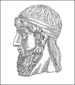
It was in the middle of this period of Athenian cultural dominance that Plato founded his famous Academy. Although we think of Plato today as a philosopher, the center of the Academy’s program was the study of mathematics. Among Plato’s discoveries were what we now call the five Platonic solids—the only convex three-dimensional shapes in which every face is an identical regular polygon.

Athenian culture spread throughout the Mediterranean, especially during the reign of Alexander the Great. Among his achievements, Alexander founded the Egyptian city of Alexandria (named for himself), which became the new center of research and learning. More than a thousand scholars worked in what we would now think of as a research institute, the Mouseion—the “Institution of the Muses”—from which we get our word “museum.” The scholars’ patrons were the Greek kings of Egypt, the Ptolemys, who paid their salaries and provided free room and board. Part of the Mouseion was the Library of Alexandria, which was given the task of collecting all the world’s knowledge. Supposedly containing 500,000 scrolls, the library kept a large staff of scribes busy copying, translating, and editing scrolls.

* * *

It was during this period that Euclid, one of the scholars at the Mouseion, wrote his Elements, one of the most important books in the history of mathematics. Elements includes derivations of fundamental results in geometry and number theory, as well as the ruler-and-compass constructions that students still learn today.

Proposition 2. If, when the less of two unequal magnitudes is continually subtracted in turn from the greater, that which is left never measures the one before it, then the two magnitudes are incommensurable.

Essentially, Euclid is saying what we observed earlier in the chapter: if our procedure for computing greatest common measure never terminates, then there is no common measure.

Euclid then goes on to explicitly describe the algorithm and prove that it computes the GCM. This diagram may be useful in following the proof:

Since this is the first algorithm termination proof in history, we’re including the entire text, using Sir Thomas Heath’s translation:

Proposition 3. Given two commensurable magnitudes, to find their greatest common measure.

Proof.

Let the two given commensurable magnitudes be AB, CD of which AB is the less; thus it is required to find the greatest common measure of AB, CD.

Now the magnitude AB either measures CD or it does not.

If then it measures it—and it measures itself also—AB is a common measure of AB, CD.

And it is manifest that it is also the greatest; for a greater magnitude than the magnitude AB will not measure AB.

Next, let AB not measure CD.

Then, if the less be continually subtracted in turn from the greater, that which is left over will sometime measure the one before it, because AB, CD are not incommensurable; [cf. X. 2] let AB, measuring ED, leave EC less than itself, let EC, measuring FB, leave AF less than itself, and let AF measure CE.

Since, then, AF measures CE, while CE measures FB, therefore AF will also measure FB.

But it measures itself also; therefore AF will also measure the whole AB.

But AB measures DE; therefore AF will also measure ED.

But it measures CE also; therefore it also measures the whole CD.

Therefore AF is a common measure of AB, CD.

I say next that it is also the greatest.

For, if not, there will be some magnitude greater than AF which will measure AB, CD.

Let it be G.

Since then G measures AB, while AB measures ED, therefore G will also measure ED.

But it measures the whole CD also; therefore G will also measure the remainder CE.

But CE measures FB; therefore G will also measure FB.

But it measures the whole AB also, and it will therefore measure the remainder AF, the greater [measuring] the less: which is impossible.

Therefore no magnitude greater than AF will measure AB, CD; therefore AF is the greatest common measure of AB, CD.

Therefore the greatest common measure of the two given commensurable magnitudes AB, CD has been found.

This “continual subtraction” approach to GCM is known as Euclid’s algorithm (or sometimes the Euclidean algorithm). It’s an iterative version of the gcm function we saw in Chapter 3. As we did before, we will use C++-like notation to show its implementation:

Click here to view code image

line_segment gcm0(line_segment a, line_segment b) {
    while (a != b) {
        if (b < a) a = a - b;
        else       b = b - a;
    }
    return a;
}

In Euclid’s world, segments cannot be zero, so we do not need this as a precondition.

Exercise 4.1. gcm0 is inefficient when one segment is much longer than the other. Come up with a more efficient implementation. Remember you can’t introduce operations that couldn’t be done by ruler-and-compass construction.

Exercise 4.2. Prove that if a segment measures two other segments, then it measures their greatest common measure.

To work toward a more efficient version of line_segment_gcm, we’ll start by rearranging, checking for b < a as long as we can:

Click here to view code image

line_segment gcm1(line_segment a, line_segment b) {
    while (a != b) {
        while (b < a) a = a - b;
        std::swap(a, b);
    }
    return a;
}

We could avoid a swap in the case where a = b, but that would require an extra test, and we’re not quite ready to optimize the code anyway. Instead, we observe that the inner while loop is computing the remainder of a and b. Let’s factor out that piece of functionality:

Click here to view code image

line_segment segment_remainder(line_segment a, line_segment b) {
    while (b < a) a = a - b;
    return a;
}

How do we know the loop will terminate? It’s not as obvious as it might appear. For example, if our definition of line_segment included the half line starting at a point and continuing infinitely in one direction, the code would not terminate. The required assumptions are encapsulated in the following axiom:

Axiom of Archimedes: For any quantities a and b, there is a natural number n such that a ≤ nb.

Essentially, what this says is that there are no infinite quantities.

* * *

Now we can rewrite our GCM function with a call to segment_remainder:

Click here to view code image

line_segment gcm(line_segment a, line_segment b) {
    while (a != b) {
        a = segment_remainder(a, b);
        std::swap(a, b);
    }
    return a;
}

So far we have refactored our code but not improved its performance. Most of the work is done in segment_remainder. To speed up that function, we will use the same idea as in Egyptian multiplication—doubling and halving our quantities. This requires knowing something about the relationship of doubled segments to remainder:

Lemma 4.1 (Recursive Remainder Lemma): If r = segment_remainder(a, 2b), then

Suppose, for example, that we wanted to find the remainder of some number n divided by 10. We’ll try to take the remainder of n divided by 20. If the result is less than 10, we’re done. If the result is between 11 and 20, we’ll take away 10 from the result and get the remainder that way.

Using this strategy, we can write our faster function:

Click here to view code image

line_segment fast_segment_remainder(line_segment a,
                                    line_segment b) {
    if (a <= b) return a;
    if (a - b <= b) return a - b;
    a = fast_segment_remainder(a, b + b);
    if (a <= b) return a;
    return a - b;
}

It’s recursive, but it’s a less intuitive form of upward recursion. In most recursive programs, we go down from n to n – 1 when we recurse; here, we’re making our argument bigger every time, going from n to 2n. It’s not obvious where the work is done, but it works.

Let’s look at an example. Suppose we have a segment a of length 45 and a segment b of length 6, and we want to find the remainder of a divided by b:

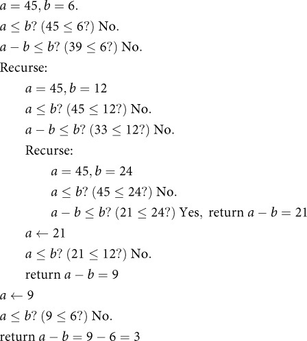
Remember that since the Greeks had no notion of a zero-length segment, their remainders were in the range [1, n].

We still have the overhead of recursion, so we’ll eventually want to come up with an iterative solution, but we’ll put that aside for now.

Finally, we can plug this code into our GCM function, providing a solution to Exercise 4.1:

Click here to view code image

line_segment fast_segment_gcm(line_segment a, line_segment b) {
    while (a != b) {
        a = fast_segment_remainder(a, b);
        std::swap(a, b);
    }
    return a;
}

Of course, no matter how fast it is, this code will still never terminate if a and b do not have a common measure.

Among the Greeks geometry was held in highest honor; nothing could outshine mathematics. But we have limited the usefulness of this art to measuring and calculating.

While there were Greek mathematicians working in Roman times, it is a remarkable fact that there is no record of any original mathematical text written in Latin (the language of ancient Rome) at that time.

The period of history that followed was not kind to the formerly great societies of Europe. In Byzantium, the Greek-speaking Eastern remnant of the former Roman Empire, mathematics was still studied, but innovation declined. By the 6th to 7th centuries, scholars still read Euclid, but usually just the first book of Elements; Latin translations didn’t even bother to include the proofs. By the end of the first millennium, if you were a European who wanted to study mathematics, you had to go to cities like Cairo, Baghdad, or Cordoba in the realm of the Arabs.

What is particularly surprising about the lack of zero outside of astronomy is that it persisted despite the fact that the abacus was well known and commonly used for commerce in nearly every ancient civilization. Abaci consist of stones or beads arranged in columns; the columns correspond to 1s, 10s, 100s, and so on, and each bead represents one unit of a given power of 10. In other words, ancient societies used a device that represented numbers in base 10 positional notation, yet there was no commonly used written representation of zero until 1000 years later.

The unification of a written form of zero with a decimal positional notation is due to early Indian mathematicians sometime around the 6th century AD. It then spread to Persia between the 6th and 9th centuries AD. Arab scholars learned the technique and spread it across their empire, from Baghdad in the east to Cordoba in the west. There is no evidence that zero was known anywhere in Europe outside this empire (even in the rest of Spain); 300 years would pass before this innovation crossed from one culture to the other.

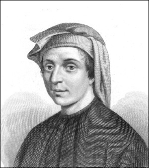
The breakthrough came in 1203 when Leonardo Pisano, also known as Fibonacci, published Liber Abaci (“The Book of Calculation”). In addition to introducing zero and positional decimal notation, this astonishing book described to Europeans, for the first time, the standard algorithms for doing arithmetic that we are now taught in elementary school: long addition, long subtraction, long multiplication, and long division. With one stroke, Leonardo brought mathematics back to Europe.

Leonardo Pisano’s later work Liber Quadratorum (“The Book of Squares”), published in 1225, is probably the greatest work on number theory in the time span between Diophantus 1000 years earlier and the great French mathematician Pierre de Fermat 400 years later. Here is one of the problems from the book:

Exercise 4.3 (easy). Prove that .

Why was a problem like this difficult for the Greeks? They had no terminating procedure for computing cube roots (in fact, it was later proven that no such process exists). So from their perspective, the problem starts out: “First, execute a nonterminating procedure....”

Leonardo’s insight will be familiar to any middle-school algebra student, but it was revolutionary in the 13th century. Basically, what he said was, “Even though I don’t know how to compute , I’ll just pretend I do and assign it an arbitrary symbol.”

Here’s another example of the kind of problem Leonardo solved:

Exercise 4.4. Prove the following proposition from Liber Quadratorum: For any odd square number x, there is an even square number y, such that x + y is a square number.

Exercise 4.5 (hard). Prove the following proposition from Liber Quadratorum: If x and y are both sums of two squares, then so is their product xy. (This is an important result that Fermat builds on.)

Zero-length segments force us to rethink our GCM and remainder procedures, because Archimedes’ axiom no longer holds—we can add a zero-length segment forever, and we’ll never exceed a nonzero segment. So we’ll allow the first argument a to be zero, but we need a precondition to ensure that the second argument b is not zero. Having zero also lets us shift our remainders to the range [0, n – 1], which will be crucial for modular arithmetic and other developments. Here’s the code:

Click here to view code image

line_segment fast_segment_remainder1(line_segment a,
                                     line_segment b) {
    // precondition: b != 0
    if (a < b) return a;
    if (a - b < b) return a - b;
    a = fast_segment_remainder1(a, b + b);
    if (a < b) return a;
    return a - b;
}

The only thing we’ve changed are the conditions; everywhere we used to say a <= b, we now check a < b.

Let’s see if we can get rid of the recursion. Every time we recurse down, we double b, so in the iterative version, we’d like to precompute the maximum amount of doubling we’ll need. We can define a function that finds the first repeated doubling of b that exceeds the difference a – b:

Click here to view code image

line_segment largest_doubling(line_segment a, line_segment b) {
    // precondition: b != 0
    while (a - b >= b) b = b + b;
    return b;
}

Now we need our iterative function to do the same computation that happens on the way out of the recursion. Each time it returns, the value of b has the value it had before the most recent recursive call (i.e., the most recent doubling). So to simulate this, the iterative version needs to repeatedly “undouble” the value, which it will do by calling a function half. Remember, we’re still “computing” with ruler and compass. Fortunately, there is a Euclidean procedure for “halving” a segment,¹ so we can use a half function. Now we can write an iterative version of remainder:

Click here to view code image

line_segment remainder(line_segment a, line_segment b) {
    // precondition: b != 0
    if (a < b) return a;
    line_segment c = largest_doubling(a, b);
    a = a - c;
    while (c != b) {
        c = half(c);
        if (c <= a) a = a - c;
    }
    return a;
}

¹ Draw a circle with the center at one end of the segment and radius equal to the segment; repeat for the other end. Use ruler to connect the two points where the circles intersect. The resulting line will bisect the original segment.

The first part of the function, which finds the largest doubling value, does what the “downward” recursion does, while the last part does what happens on the way back up out of the recursive calls. Let’s look again at our example of finding the remainder of 45 divided by 6, this time with the new remainder function:

Notice that the successive values of c in the iterative implementation are the same as the values of b following each recursive call in the recursive implementation. Also, compare this to the trace of our earlier version of the algorithm at the end of Section 4.2. Observe how the results of the first part (c = 24 and a = 21) here are the same as the innermost recursion in the old example.

This is an extremely efficient algorithm, nearly as fast as the hardware implemented remainder operation in modern processors.

* * *

What if we wanted to compute quotient instead of remainder? It turns out that the code is almost the same. All we need are a couple of minor modifications, shown in bold:

Click here to view code image

integer quotient(line_segment a, line_segment b) {
    // Precondition: b > 0
    if (a < b) return integer(0);
    line_segment c = largest_doubling(a, b);
    integer n(1);
    a = a - c;
    while (c != b) {
        c = half(c); n = n + n;
        if (c <= a) { a = a - c; n = n + 1; }
    }
    return n;
}

Quotient is the number of times one line segment fits into another, so we use the type integer to represent this count. Basically, we are going to count multiples of b. If a < b, then we don’t have any multiples of b and we return 0. But if a ≥ b, we initialize the counter to 1, then double it each time we halve c, adding one more multiple for each iteration when it fits. Again, let’s work through an example. This time, instead of finding the remainder of 45 divided by 6, we’ll find the quotient of 45 divided by 6.

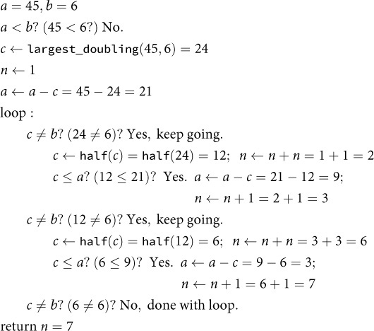
Essentially, this is the Egyptian multiplication algorithm in reverse. And Ahmes knew it: a primitive variant of this algorithm, known to the Greeks as Egyptian division, appears in the Rhind papyrus.

Click here to view code image

std::pair<integer, line_segment>
quotient_remainder(line_segment a, line_segment b) {
    // Precondition: b > 0
    if (a < b) return {integer(0), a};
    line_segment c = largest_doubling(a, b);
    integer n(1);
    a = a - c;
    while (c != b) {
        c = half(c); n = n + n;
        if (c <= a) { a = a - c; n = n + 1; }
    }
    return {n, a};
}

In fact, any quotient or remainder function does nearly all the work of the other.

Most computing architectures, whether ruler-and-compass or modern CPUs, provide an easy way to compute half; for us, it’s just a 1-bit right shift. However, if you should happen to be working with an architecture that doesn’t support this functionality, there is a remarkable version of the remainder function developed by Robert Floyd and Donald Knuth that does not require halving. It’s based on the idea of the Fibonacci sequence—another of Leonardo Pisano’s inventions, which we will discuss more in Chapter 7. Instead of the next number being double the previous one, we’ll make the next number be the sum of the two previous ones:²

Click here to view code image

line_segment remainder_fibonacci(line_segment a, line_segment b) {
    // Precondition: b > 0
    if (a < b) return a;
    line_segment c = b;
    do {
        line_segment tmp = c; c = b + c; b = tmp;
    } while (a >= c);
    do {
        if (a >= b) a = a - b;
        line_segment tmp = c - b; c = b; b = tmp;
    } while (b < c);

    return a;
}

² Note that this sequence starts at b, so the values will not be the same as the traditional Fibonacci sequence.

The first loop is equivalent to computing largest_doubling in our previous algorithm. The second loop corresponds to the “halving” part of the code. But instead of halving, we use subtraction to get back the earlier number in the Fibonacci sequence. This works because we always keep one previous value around in a temporary variable.

Exercise 4.6. Trace the remainder_fibonacci algorithm as it computes the remainder of 45 and 6, in the way we traced the remainder algorithm in Section 4.5.

Exercise 4.7. Design quotient_fibonacci and quotient_remainder_fibonacci.

Now that we have an efficient implementation of the remainder function, we can return to our original problem, the greatest common measure. Using our new remainder function from p. 54, we can rewrite Euclid’s algorithm like this:

Click here to view code image

line_segment gcm_remainder(line_segment a, line_segment b) {
    while (b != line_segment(0)) {
        a = remainder(a, b);
        std::swap(a, b);
    }
    return a;
}

Since we now allow remainder to return zero, the termination condition for the main loop is when b (the previous iteration’s remainder) is zero, instead of comparing a and b as we did originally.

We will use this algorithm for the next few chapters, leaving its structure intact but exploring how it applies to different types. We will leave our ruler-and-compass constructions behind and implement the algorithm with a digital computer in mind. For example, for integers, the equivalent function is the greatest common divisor (GCD):

Click here to view code image

integer gcd(integer a, integer b) {
    while (b != integer(0)) {
        a = a % b;
        std::swap(a, b);
    }
    return a;
}

The code is identical, except that we have replaced line_segment with integer and used the modulus operator % to compute the remainder. Since computers have instructions to compute the integer remainder (as invoked by the C++ modulus operator), it’s better to use them than to rely on doubling and halving.

To prove that the algorithm terminates, we rely on the fact that

0 ≤ (a mod b) < b

Therefore, in each iteration, the remainder gets smaller. Since any decreasing sequence of positive integers is finite, the algorithm must terminate.

To prove that the algorithm computes the GCD, we start by observing that in each iteration, the algorithm computes a remainder of a and b, which by definition is

r = a – bq

where q is the integer quotient of a divided by b. Since gcd(a, b) by definition divides a and also divides b (and therefore bq), it must also divide r. We can rewrite the remainder equation as follows:

a = bq + r

By the same reasoning, since gcd(b, r) by definition divides b (and therefore bq), and also divides r, it must also divide a. Since pairs (a, b) and (b, r) have the same common divisors, they have the same greatest common divisor. Therefore we have shown that

At each iteration, the algorithm replaces gcd(a, b) with gcd(b, r) by taking the remainder and swapping the arguments. Here is the list of remainders, starting with a₀ and b₀, the initial arguments to the function:

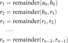
Using the definition of remainder, we rewrite the sequence computed by the algorithm like this:

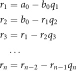
What Equation 4.1 guarantees is that the GCD stays the same each time. In other words:

gcd(a₀, b₀) = gcd(b₀, r₁) = gcd(r₁, r₂) = ··· = gcd(r_n–1, r_n)

But we know that the remainder of r_n-1 and r_n is 0, because that’s what triggers the termination of the algorithm. And gcd(x, 0) = x. So

gcd(a₀, b₀) = ··· = gcd(r_n–1, r_n) = gcd(r_n, 0) = r_n

which is the value returned by the algorithm. Therefore, the algorithm computes the GCD of its original arguments.