
Chapter 17. Monte Carlo Photon Transport on the GPU
László Szirmay-Kalos, Balázs Tóth and Milán Magdics
This chapter presents a fast parallel Monte Carlo method to solve the radiative transport equation in inhomogeneous participating media for light and gamma photons. Light transport is relevant in computer graphics while higher-energy gamma photons play an essential role in medical or physical simulation. Real-time graphics applications are speed critical because we need to render more than 20 images per second in order to provide the illusion of continuous motion. Fast simulation is also important in interactive systems like radiotherapy or physical experiment design where the user is allowed to place the source and expects an instant feedback about the resulting radiation distribution. The speed of multiple scattering simulation is also crucial in iterative tomography reconstruction where the scattered radiation is estimated from the actually reconstructed data, removed from the measurements, and reconstruction is continued for the residual that is assumed to represent only the unscattered component.
17.1. Physics of Photon Transport
Computing multiple scattering and rendering inhomogeneous participating media in a realistic way are challenging problems. The most accurate approaches are based on Monte Carlo quadrature and simulate the physical phenomena by tracing photons randomly in the medium and summing up their contribution.
The conditional probability density that a photon collides with the particles of the material provided that the photon arrived at this point is defined by the
extinction coefficient
 , which may depend on the photon's frequency
 and also on the location
 if the particle density is not homogeneous. The extinction coefficient can usually be expressed by the product of the material density
 and a factor depending just on the frequency.
Upon collision, the photon may get reflected or absorbed. The probability of reflection is called the
albedo
and is denoted by
 .
.
The random reflection direction is characterized by two spherical coordinates,
scattering angle
 and
azimuth angle
and
azimuth angle
 (Figure 17.1
). The probability density of
scattering angle
(Figure 17.1
). The probability density of
scattering angle
 that is between the original and the new directions may depend on the frequency and is described by the physical model (we use the
Rayleigh scattering
[12]
model for light photons and the
Klein-Nishina formula
[11]
,
[13]
for gamma photons). The probability density of the azimuth angle is uniform due to the rotational symmetry.
that is between the original and the new directions may depend on the frequency and is described by the physical model (we use the
Rayleigh scattering
[12]
model for light photons and the
Klein-Nishina formula
[11]
,
[13]
for gamma photons). The probability density of the azimuth angle is uniform due to the rotational symmetry.
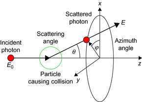 |
| Figure 17.1
Photon scattering in participating media. The incident photon of energy
|
The photon's energy
 is proportional to its frequency and the ratio of the proportionality is the
Planck constant
is proportional to its frequency and the ratio of the proportionality is the
Planck constant
 . The energy (i.e., the frequency of a higher energy gamma photon) may change as a result of scattering. According to the Compton law, there is a unique correspondence between the scattering angle and the relative change of the photon energy:
 where
where
 is the scattered photon energy,
 is the incident photon energy,
 is the rest mass of the electron, and
 is the speed of light. Examining the Compton formula, we can conclude that the energy change at scattering is significant when
 is nonnegligible with respect to the energy of the electron
 . This is not the case for photons of visible wavelengths, when
 ; thus, their scattered energy will be similar to the incident energy. Consequently, we can decompose the simulation of low-energy radiation (light photons) to different frequencies, but on higher energies (gamma photons), the frequency will be an attribute of each simulated photon.
In computer simulation, the photon is traced according to the basic laws mentioned so far. The inputs of the simulation are the density of the participating medium, which is defined by a 3-D scalar density field
 , the frequency dependent albedo function, and the probability density of the scattering angle. The density field is assumed to be available in a discrete form as a 3-D texture of voxels. The frequency dependent albedo and scattering density functions may be defined either by tables stored in textures or by algebraic formulae.
In order to simulate the photon transport process, the collision, the absorption, and the scattering direction should be generated with the probability densities defined by the physical model. One approach to generate random variables with prescribed probability densities is the
inversion method
. The inversion method first calculates the
cumulative probability distribution
(CDF
) as the integral of the probability density and then generates the discrete samples by inverting the CDF for values that
are uniformly distributed in the unit interval. Formally, if the cumulative probability distribution of a random variable is
 , then a random sample
 can be generated by solving equation
 where
where
 is a random variable uniformly distributed in the unit interval and is usually obtained by calling the random number generator.
17.2. Photon Transport on the GPU
Photons travel in space independently of each other and thus can be simulated in parallel, thereby revealing the inherent parallelism of the physical simulation (nature is a massively parallel machine). The algorithm of simulating the path of a single photon is a nested loop. Both the outer and the inner loops are dynamic, and their number of executions cannot be predicted. The body of the outer loop is responsible for finding the next scattering point, then sampling absorption and the new scattering direction in case of survival. This loop is terminated when the photon is absorbed or it leaves the simulation volume. The number of scattering events of different photons will range on a large interval, and so will the number of outer loop executions. The inner loop visits voxels until the next scattering point is located; this process depends on the drawn random number and also on the density of medium along the ray of the photon path. Both the random number and the density vary, thus again the number of visited voxels may be different for different samples (Figure 17.2
).
 |
| Figure 17.2
Causes of control path divergence in photon transport simulation. A photon path has a random number of scattering points and between two scattering points there may be a different number of voxels.
|
The problem of executing different numbers of iterations in parallel threads becomes crucial on the GPU. If we assigned a photon to a computational thread of the GPU, then the longest photon path and the longest ray of all paths in each warp will limit the computational speed. In order to maintain warp coherence, the execution lengths of the threads must be similar, and the threads are preferred to
always execute the same instruction sequence. To attack these problems, we restructure the transport simulation according to the requirements of efficient GPU execution; that is, we develop algorithms that can be implemented with minimal conditional instructions.
To solve the problem of different numbers of scattering events, we iterate photon steps, that is, rays in computational threads. A step includes identifying the next scattering point, making the decision on termination, and sampling the new direction if the photon survived the collision, or generating a new photon at the source otherwise. This strategy keeps all threads busy at all times.
After this restructuring, threads may still diverge. Determining whether the photon is absorbed and sampling the new scattering direction are based on the local properties of the medium; thus, these tasks require the solution of an equation that contains just a few variables, which can be determined from the actual position. Even this simple problem becomes difficult if the CDF cannot be analytically computed and symbolically inverted. In these cases, numerical methods should be used. Free path sampling is even worse because it requires the exploration of a larger part of the medium, which corresponds to a lot of memory accesses being relatively slow on current GPUs. Both iterative numerical root finding and the exploration of the volume in regions of different density lead to thread divergence and eventually poor GPU utilization.
As different photons are traced randomly, they visit different parts of the simulated volume, resulting in parallel accesses of far parts of the data memory. This kind of memory accesses degrades cache utilization. To solve this problem, one might propose the assignment of those photons to a warp that possibly has similar paths. Because random paths are computed from sequences of uniformly distributed random numbers, this would mean the clustering of vectors of random numbers. A complete path may be associated with many (e.g., more than 20) random numbers, so the clustering operation should work in very high dimensional spaces, which is not feasible in practice. So photons are sorted according to only the first random number and assigned to warps in the sorted sequence. This step provides little initial data access coherence, but sooner or later, threads will inevitably fetch different parts of the volume.
In order to guarantee the coherence of threads tracing rays in the medium, we develop a conditional instruction-free solution for sampling absorption and scattering direction. To solve the free-path-sampling problem and also to limit the data access divergence, we present a technique that uses a low-resolution voxel array in addition to the original high-resolution voxel array. This technique significantly reduces the number of texture fetches to the high-resolution array as well as the number of iterations needed to find the next scattering point.
17.2.1. Free Path Sampling
The first step of simulating a photon of current location
 , direction
 , and frequency
 is the sampling of the
free path
is the sampling of the
free path
 that the photon can fly without collision, that is, the determination of the next interaction point along the ray
 of its path. The probability density that photon-particle collision happens is the extinction coefficient. From this, the cumulative probability distribution of the free path length can be expressed in the form of an exponential decay; thus free path sampling is equivalent to the solution of the following equation for scalar
 that is uniformly distributed in the unit interval:
The integral of the extinction coefficient is called the
optical depth
, for which the following equation can be derived:
(17.1)
Free path sampling, that is, the solution of this equation, is simple when the medium is homogeneous; in other words, when the extinction coefficient is the same everywhere:
When the medium is inhomogeneous, the extinction coefficient is not constant but is represented by a voxel array. In this case, the usual approach is
ray marching
that takes small steps
 along the ray and finds step number
 when the Riemann sum approximation of the optical depth gets larger than
 :
:
Step size
 is set to the edge length of the voxel in order not to skip voxels during the traversal. Unfortunately, this algorithm requires a lot of voxel array fetches, especially when the voxel array is large and the average extinction is small. To make it even worse, the number of texture fetches vary significantly, depending on the random length of the ray. Recall that free path sampling is the evaluation of a simple formula when the optical depth is a simple algebraic expression, as in the case of homogeneous volumes. However, if the optical depth can be computed only from many data, which happens when the extinction coefficient is specified by a high-resolution voxel array, then the sampling process will be slow. Fortunately, we do not have to pay the full cost if we have at least partial information about the extinction coefficient, which can be utilized to reduce the number of fetches. This is the basic idea of our method.
Free path sampling is equivalent to the solution of
Eq. 17.1
for path length
s
, where we want to replace the optical depth by a simpler function that can be computed from a few variables. To reach this goal, we modify the volume by adding virtual “material” or particles in a way that the total density will follow a simple function. One might think that mixing additional material into the original medium would also change the radiation intensity inside the volume, resulting in a bad solution, which is obviously not desired. Fortunately, this is not necessarily the case if the other two free properties of the virtual material — namely the albedo and the probability density of the scattering angle — are appropriately defined.
Virtual particles must not alter the radiation intensity inside the medium; that is, they must not change the energy and the direction of photons during scattering. This requirement is met if the virtual particle has
albedo
1, that is, it reflects photons with probability 1, and the probability density of the scattering angle is a Dirac-delta at zero — in other words, it does not change the photon's direction with probability 1.
More formally, we handle heterogeneous volumes by mixing additional virtual particles into the medium to augment the extinction coefficient to a simpler upper-bounding function
 . For
original extinction coefficient
. For
original extinction coefficient
 , we have to find the extinction coefficient
 of the virtual particles so that in the
combined medium
of real and virtual particles the extinction coefficient is
of the virtual particles so that in the
combined medium
of real and virtual particles the extinction coefficient is
 .
.
When a collision occurs in the combined medium, we have to determine whether it happened on a real or on a virtual particle. Sampling is required to generate random points with a prescribed probability density, and therefore, it is enough to solve this problem randomly with the proper probabilities. As the extinction parameters define the probability density of scattering, ratios
 and
and
 give us the probabilities whether scattering happened on a real or on a virtual particle, respectively.
Having added the virtual particles, we can execute free path sampling in the following steps (Figure 17.3
):
1. Generate tentative path length
 and
tentative collision point
and
tentative collision point
 using the upper-bounding extinction coefficient function
 . This requires the solution of the sampling equation using the maximum extinction:

(17.2)
2. When a tentative collision point
 is identified, we decide randomly with probability
 whether scattering happened on a real or on a virtual particle. If only virtual scattering occurred, then the particle's direction is not altered and a similar sampling step is repeated from the scattering point. This loop is terminated when a real scattering is found.
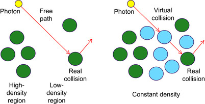 |
| Figure 17.3
The application of virtual particles. In the left image the free path sampling of the original volume of real particles (colored as light gray) is shown. The right image depicts the total volume containing both the real and the virtual (dark gray) particles. Collision with a virtual particle does not alter the photon direction.
|
Note that the samples declared as real by the algorithm are generated with a conditional probability density of the original extinction coefficient no matter what upper-bounding extinction coefficient is built into the sampling. However, the efficiency of the sampling is greatly affected by the proper choice of the upper-bounding coefficient. On one hand, the upper-bounding coefficient should offer a simple
solution for
Eq. 17.2
. On the other hand, if the difference of the upper-bounding coefficient and the real coefficient, that is, the density of virtual particles, is high, then the probability of virtual scattering events will also be high, thus requiring many additional sampling steps until the real scattering is found. Thus, an optimal upper-bounding coefficient offers an easy solution of
Eq. 17.2
and is a tight upper bound of the real extinction coefficient.
To find a simple, but reasonably accurate upper bound, we use a piecewise constant function that is defined in a low-resolution grid of
macrocell
s (Figure 17.4
) as proposed in
[8]
and assign the maximum extinction coefficient of its original voxels to each macrocell. If only one macrocell is defined that contains the whole volume, then the method becomes equivalent to
Woodcock tracking
[10]
.
 |
| Figure 17.4
Free path sampling with virtual particles. We execute a 3-D DDA voxel traversal in the grid of macrocells and analytically obtain the optical depth
|
In order to solve
Eq. 17.2
, we execute a 3-D DDA-like voxel traversal
[4]
on the macrocell grid to visit all macrocells that are intersected by the ray. The 3-D DDA algorithm is based on the recognition that the boundaries of the cells are on three collections of parallel planes, which are orthogonal to the respective coordinate axes. The algorithm maintains three ray parameters representing the next intersection points with these plane collections. The minimum of the three ray parameters represents the exit point of the current cell. To step on to the next cell, an increment is added to this ray parameter. The increments corresponding to the three plane collections are constants for a given ray and should be calculated only once.
During traversal, ray parameters
 corresponding to points when the ray crosses the macrocell boundaries are found. We visit macrocells one by one until the current macrocell contains the root of
Eq. 17.2
(Figure 17.4
).
corresponding to points when the ray crosses the macrocell boundaries are found. We visit macrocells one by one until the current macrocell contains the root of
Eq. 17.2
(Figure 17.4
).
The inequalities selecting the macrocell
 that contains the scattering point are:
 where
where
 is the constant extinction coefficient of the augmented volume in macrocell
 .
.
The important differences of ray marching and the proposed approach are that steps
 are not constant but are obtained as the length of the intersection of the ray and the macrocells.
When in step
 the inequalities are first satisfied, the macrocell of the scattering point is located. As
 is constant in the identified macrocell, its integral in
Eq. 17.2
is linear; thus, the free path sampling becomes equivalent to the solution of a linear equation:
is constant in the identified macrocell, its integral in
Eq. 17.2
is linear; thus, the free path sampling becomes equivalent to the solution of a linear equation:

The proposed free-path-sampling method causes significantly smaller warp divergence than ray marching or Woodcock tracking. In ray marching, the number of iteration cycles would be proportional to the length of the free path, which may range from 1 to the linear resolution of the voxel array (e.g., 512). In Woodcock tracking, the average step size is inversely proportional to the global maximum of the extinction coefficient. The probability of nonvirtual collisions is equal to the ratio of the actual and the maximum extinction coefficients, so the algorithm would take many small steps and find only virtual collisions in low-density regions. In the proposed method, however, the probability of nonvirtual collisions is the ratio of actual coefficient and the maximum of this macrocell, so it corresponds to how accurately the piecewise constant bound of macrocells represents the true extinction coefficient. Increasing the resolution of the macrocell grid, this accuracy can be controlled paying the price of more macrocell steps. For example, in the head dataset (Figure 17.9
) of
 voxels, with
 macrocell grid resolution, the average number of virtual collisions before finding a real one is 0.95, whereas the average number of macrocell steps is 1.7. If the macrocell resolution is increased to
 , then the average number of virtual collisions reduces to 0.92, but the average number of visited macrocells increases to 3.7. Generally, very few (at the most one or two virtual collisions) may happen before finding the real collision point, and the possible number of macrocell steps is far smaller than that of the steps of a ray-marching algorithm.
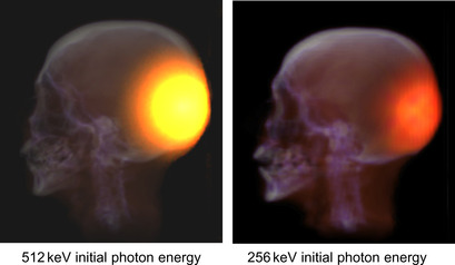 |
| Figure 17.9
Visualization of the radiation dose owing to gamma photon transfer. The volume is defined by a
|
17.2.2. Absorption Sampling
When the photon collides with a real particle, we should determine whether or not absorption happened and also the new direction if the photon survived the collision. The probability of survival is defined by the albedo; thus, this random decision is made by checking whether the albedo is larger than a random number uniformly distributed in the unit interval:

In our implementation the frequency dependent albedo function is stored in a 1-D texture addressed by the frequency normalized by maximum frequency
 that is the frequency of emitted photons. Turning linear interpolation on, the albedo is smoothly interpolated in between the representative frequencies. For light photons, the albedo is stored just on the frequencies corresponding to the red, green, and blue light.
17.2.3. Scattering Direction
If the photon survives the collision, a new continuation direction needs to be sampled, which is defined by scattering angle
 and azimuth angle
 .
.
The azimuth angle
 is uniformly distributed; thus, it is generated as
 where
where
 is a uniform random number in the unit interval. The scattering angle is sampled by solving the sampling equation
 where
where
 is the cumulative probability distribution of the cosine of the scattering angle on a given frequency, and
 is another uniform random number. The probability density of the scattering angle is usually defined by the physical model and is a moderately complex algebraic expression (we use Rayleigh scattering for light photons and the Klein-Nishina differential cross section for gamma photons, but other phase functions can also be handled in the discussed way), from which the cumulative distribution can be obtained by integration. Unfortunately, for most of the models, the integral cannot be expressed in a closed form, and the sampling equation cannot be solved analytically. On the other hand, numerical solutions, like the midpoint or the false position methods, would execute a loop and would be slow.
To attack this problem, we find regularly placed samples for
 and
and
 , and solve the sampling equation for these samples offline (we set
 and
and
 to 128). The solutions are stored in a 2-D texture that can be addressed by
 and
and
 . The content of this texture is the cosine of the scattering angle corresponding to the given frequency and random number (Figure 17.5
). During the simulation, we just obtain the cosine of the sampling direction by
looking up this texture addressed by the current values of the uniform random number and the photon frequency. Because for light photons the scattering angle is independent of the frequency, we can use just a 1-D texture for the solutions of the sampling problem.
. The content of this texture is the cosine of the scattering angle corresponding to the given frequency and random number (Figure 17.5
). During the simulation, we just obtain the cosine of the sampling direction by
looking up this texture addressed by the current values of the uniform random number and the photon frequency. Because for light photons the scattering angle is independent of the frequency, we can use just a 1-D texture for the solutions of the sampling problem.
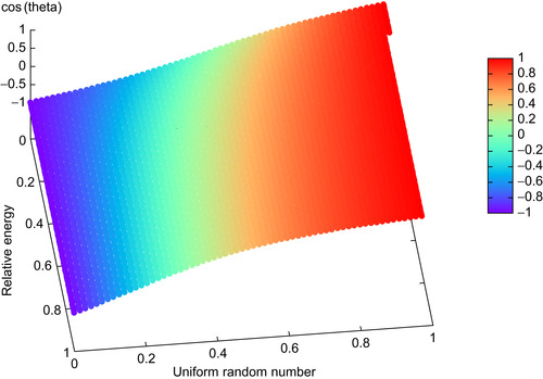 |
| Figure 17.5
The table used for the sampling of the scattering angle assuming Compton scattering and the Klein-Nishina phase function. The table is parameterized with a random variable uniformly distributed in [0,1] and the relative energy of the photon with respect to the energy of the electron (512 keV), and provides the cosine of the scattering angle.
|
17.2.4. Parallel Random Number Generation
All discussed sampling steps transform random numbers that are uniformly distributed in the unit interval. Free path sampling needs as many random numbers as virtual scattering events happen until the first real scattering point. Absorption sampling requires just one additional random variable, but direction sampling uses two. Because different steps of the photon path are statistically independent, every step should use a new set of random numbers. Furthermore, different photons behave statistically independently, and therefore, the simulation of every photon should be based on a new random number sequence. Clearly, if we used the same random number generator in all parallel threads simulating different photons, then we would unnecessarily repeat the very same computation many times.
The typical solution of this problem is the allocation of a private random number generator for each parallel thread. To guarantee that their sequences are independent, the private random number generators are initialized with random seeds. The private random number generators run on the GPU and are assigned to parallel threads, whereas their random initial seeds are generated on the CPU using the random number generator of the C library.
We note that the mathematical analysis and the construction of robust parallel random number generators (and even nonparallel ones) are hard problems, which are out of the scope of this chapter. The interested reader should consult the literature, for example, a CUDA implementation
[6]
, which is also used in our program, and
[7]
for the mathematical background.
17.3. The Complete System
The discussed method has been integrated into a photon-mapping global illumination application, which decomposes the rendering into a shooting and a gathering phase. During shooting, multiple scattering of photons is calculated in the volume, registering the collision points, photon powers, and incident directions. The powers of photon hits are accumulated in cells defined by a 3-D array called the
illumination buffer
. The gathering phase visualizes the illumination buffer by standard alpha blending.
The inputs of the simulation system are the position of the isotropic radiation source, the position of the virtual camera, and the three-dimensional texture of the density field.
The shooting phase iteratively updates three arrays (Figure 17.6
):
1. The one-dimensional
seed buffer
that stores the seeds of the parallel random number generators. This buffer is initialized by the CPU and is updated when a new random number is generated by its respective thread.
2. The one-dimensional
photon buffer
representing the currently simulated photons with their current position, direction, and energy.
3. The three-dimensional
illumination buffer
.
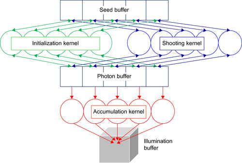 |
| Figure 17.6
The architecture of the shooting phase of the simulation program. A thread is built of three functions: initialization, shooting, and accumulation. The seed buffer contains the seeds of the random number generators, which are initialized by the CPU and are updated by the initialization and the shooting functions. The initialization function processes the photon buffer and executes two operations, depending on whether the photon exists and is alive. It samples the scattering direction of already existing and living photons, and sets the initial position and direction of newly born ones that replace the dead photons. The shooting function finds the next collision location and decides on termination. A thread is assigned to its own items of the seed buffer and the photon buffer, so no synchronization is needed here. The accumulation function adds the power of the photon to a cell of the illumination buffer selected by the photon's location.
|
The photon buffer and the seed buffer have the same size, which is equal to the number of concurrently simulated photons, that is, the number of threads, and there is a one-to-one mapping between the threads and the items of the photon buffer and the seed buffer.
The photon buffer is managed by three functions of the thread that are called in a cyclic manner:
1. The
initialization function
puts newly emitted photons into the places of dead or uninitialized photons in the photon buffer and samples the scattering direction of existing or living ones. In the place of dead photons, a new photon is generated at the position of the source with uniformly distributed random direction and assigning the source's energy level to the photon. If the photon already exists and is alive, then its position is not altered, but a new scattering direction is sampled, and its energy level is modified according to the Compton law. Generating a new photon and sampling the scattering direction may seem conceptually different, but these processes have very similar control paths. Both types of random direction sampling require two new uniform random numbers in the unit interval. If the scattering is uniform, then the only difference is that the location of newly born photons is set to the source position. In the general case, the different formulae of initial direction and scattering direction may cause small warp divergence.
2.
The
shooting function
simulates one step of the photons stored in the photon buffer. It calculates the next scattering event of its own photon executing free path sampling and then decides whether absorption occurs. If the photon leaves the volume without collision, or the absorption check tells us that the photon is absorbed, then its status is set to “dead,” to get the next initialization operation to generate a new emitted photon in its place. The thread finally writes out the modified location and the status of the photon.
3. The
accumulation function
gathers the incident photon powers from the photon buffer and adds them to the illumination buffer shared by all threads. The illumination buffer is a 3D grid, where an item represents the total irradiance arriving at the respective grid cell. The quantized Cartesian coordinates of the photon's actual position serves as an index into the accumulation buffer where the incident power is added. Not only scattered photons but also absorbed photons are considered because they also arrived at this point. Note that this is the only place in our algorithm where different threads may write to the same memory location, and synchronization problems might occur. The correct implementation requires semaphores or atomic add operations to guarantee that no photon power gets lost. If we remove the mutual exclusion, then the power of some photons may not be added to the buffer. As the number of active threads is far smaller than the number of data items in the illumination buffer, the probability of such missing photons is rather small. Moreover, the simulation process will trace millions of photons, so a few missing photons cause just a negligible error.
For the visualization of the simulation results, we implemented two methods. The first option assigns a pseudocolor to each illumination buffer item, which is determined by the
irradiance
, and renders the volume with standard alpha blending. This kind of visualization is appropriate in medical systems where we are interested in the radiation dose of body tissues. Irradiance
 is computed from the in-scattered flux
[5]
:
is computed from the in-scattered flux
[5]
:
 where
where
 is the power of the
 th photon arriving at this cell, and
 is the volume of the cell. In order to visualize not only the total energy but also the spectrum, a separate irrandiance value is computed in different frequency ranges, and a photon is added only to that irradiance where its frequency fits.
The second method computes the radiance arriving at a virtual camera and can be used, for example, in global illumination rendering. To compute the radiance, the irradiance is multiplied by the albedo of the material, and the probability density that the inscattered photon gets reflected to the direction of the virtual camera.
17.4. Results and Evaluation
The implementation of the discussed method is based on CUDA and runs entirely on the GPU. We tested the system on an NVIDIA GeForce 260 GTX graphics card. The current version assumes a single isotropic point source and runs on a single GPU, but the extension to more general sources and the exploitation of multi-GPU cards and GPU clusters are straightforward. In our application the
radiation source can be placed interactively in the volume represented by a 3-D texture fitting into the GPU texture memory.
Simulations executed by our photon transport program at interactive rates can also be done by commercially available and widely used Monte Carlo tools, like Geant4
[2]
, GATE (http://www.opengatecollaboration.org
), MCNP (http://mcnp-green.lanl.gov/
), SimSet (http://depts.washington.edu/simset
), or PeneloPET
[3]
, but the computation of the same problem in these systems takes hours or even days.
An optimized, multithreaded CPU (Intel Q8200) program is able to trace 0.4 million photons in each second with Woodcock tracking according to
[14]
. Our implementation simulates 36 million and 166 million photons in a second on NVIDIA GeForce 260 GTX and NVidia GeForce 480 GTX GPUs; these rates correspond to 90 times and 415 times speedups, respectively. The shares of the main functions in the execution time are 30% for initialization, 60% for shooting, and 10% for accumulation. According to the profiler results, the GPU program is memory bandwidth bound.
We used the GATE package to validate our program. We took the same density field and simulated the photon transport, and then finally compared the results. Of course, in a Monte Carlo simulation we cannot expect the two results to be exactly the same; thus, we also computed the variance of the results and checked whether the difference is smaller than the standard deviation. For light photons, there is another possibility for validation. If the medium is optically dense, then the diffusion equation is a good approximation of the radiance transfer, which can be solved analytically for homogeneous medium and a single isotropic radiation source
[9]
. Our application has passed both tests.
Figures 17.7
and
17.8
show the rendering results of our program when light photons are transported. The images show the radiance levels encoded by pseudocolor superimposed onto the image of the density field. Generally, the error of Monte Carlo methods is inversely proportional to the square root of the number of simulated paths, whereas the rendering time is proportional to the number of paths. In our implementation, noisy initial results are generated at high-frame rates, and even visually converged images (the relative error is less than 1%) are obtained at interactive speed.
 |
| Figure 17.7
Visualization of the radiation dose caused by a point source emitting lower energy photons in isotropic material. The volumes are defined by
|
 |
| Figure 17.8
Visualization of the radiation dose caused by a point source emitting lower-energy photons in isotropic material. The volume is defined by a
|
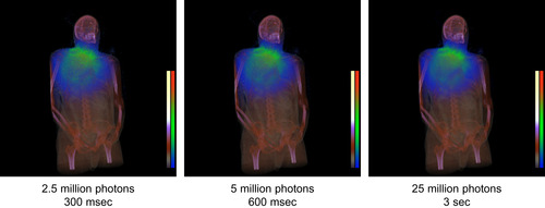
Figure 17.8
demonstrates that the method scales well for higher-resolution models as well. Here, the density is taken from the visible human dataset converted to a
 resolution voxel array. Volumes of this size are the largest that fit into the memory of our GPU.
Figure 17.9
depicts the results of gamma photon transport assuming two different sources emitting photons on 512 keV and 256 keV energy levels, respectively. Note that the simulation time of gamma photons is practically the same as for light photons, although the equations are slightly more complicated.
17.5. Future Directions
The presented implementation has several limitations that were necessary to keep the system simple and small. For example, the Rayleigh and Klein-Nishina models are hardwired into the code, so is the single isotropic source that emits either 512 keV photons or a photon triplet on the frequencies of red, green, and blue colors. Although, these settings are very common, the 512 keV level corresponds to positron-electron annihilation, while the light photon triplet to the standard selection in computer graphics, a more general user interface could widen the field of applications.
The limitation that the density field should fit into the GPU memory is even more challenging. Because our proposed method accesses the high-resolution array just to decide whether a real collision happened and otherwise uses only the low-resolution array of macrocells, it is a natural extension to store only the low-resolution array of macrocells in the GPU memory and copy the real extinction coefficients from the CPU memory only when they are needed. This extension would allow practically arbitrarily high-resolution models to be simulated; these models are badly needed in medical diagnosis. However, the data access pattern of the high-resolution array is very incoherent, so realizing a caching scheme for it in the GPU memory is not simple. We consider this as our most important future work.
Another possibility is the consideration of procedurally generated models, which represent the high-resolution model as an algorithm instead of a high-resolution array. For such models, arbitrary virtual resolutions can be achieved.
References
[1]
K. Assie, B. Breton,
et al.
,
Monte Carlo simulation in PET and SPECT instrumentation using GATE
,
Nucl. Instrum. Methods Phy. Res.
527
(1–2
) (2004
)
180
–
189
.
[2]
Geant, Physics Reference Manual, Version 4 9.1, CERN (2007) (Technical report).
[3]
S. Espana, J. Herraiz,
et al.
,
PeneloPET, a monte carlo PET simulation toolkit based on PENELOPE: features and validation
,
In:
IEEE Nuclear Science Symposium Conference
(2006
)
IEEE
, pp.
2597
–
2601
.
[4]
A. Fujimoto, T. Takayuki, I. Kansei,
Arts: accelerated ray-tracing system
,
IEEE Comput. Graph. Appl.
6
(4
) (1986
)
16
–
26
.
[5]
H.W. Jensen, P.H. Christensen,
Efficient simulation of light transport in scenes with participating media using photon maps
,
In:
Proceedings of SIGGRAPH ’98
(1998
), pp.
311
–
320
.
[6]
L. Howes, D. Thomas,
Efficient random number generation and application using CUDA
,
In:
GPU Gems
,
3
(2007
)
Addison Wesley
,
Upper Saddle Creek
.
[7]
D.E. Knuth,
The Art of Computer Programming
.
vol. 2 (Seminumerical Algorithms)
(1981
)
Addison-Wesley
,
Upper Saddle Creek
.
[8]
L. Szirmay-Kalos, B. Tóth, M. Magdics, B. Csébfalvi,
Efficient free path sampling in inhomogeneous media, Poster from Eurographics
. (3–7 May, 2010
)
Norrköping
,
Sweden
.
[9]
L. Szirmay-Kalos, G. Liktor, T. Umenhoffer, B. Tóth, S. Kumar, G. Lupton, Parallel iteration to the radiative transport in inhomogeneous media with bootstrapping, IEEE Trans. Vis. Comput. Graph. (in press).
[10]
E. Woodcock, T. Murphy, P. Hemmings, S. Longworth,
Techniques used in the GEM code for Monte Carlo neutronics calculation
,
In:
Proceedings of the Conference Applications of Computing Methods to Reactors, ANL-7050
(1965
)
.
[11]
C.N. Yang,
The Klein-Nishina formula & quantum electrodynamics
,
Lect. Notes Phys.
746
(2008
)
393
–
397
.
[14]
A. Wirth, A. Cserkaszky, B. Kári, D. Légrády, S. Fehér, S. Czifrus,
et al.
,
Implementation of 3D Monte Carlo PET reconstruction algorithm on GPU
,
In:
IEEE Medical Imaging Conference ’09
IEEE, The Nuclear and Plasma Sciences Society of the Institute of Electrical and Electronic Engineers, 25-31 October, Orlando, FL
. (2009
), pp.
4106
–
4109
.
..................Content has been hidden....................
You can't read the all page of ebook, please click here login for view all page.