
Chapter 18. High-Performance Iterated Function Systems
Christoph Schied, Johannes Hanika, Holger Dammertz and HendrikP.A. Lensch
This chapter presents an interactive implementation of the Fractal Flames algorithm which is used to create intriguing images such as
Figure 18.1
. It uses CUDA and OpenGL to take advantage of the computational power of modern graphics cards. GPUs use a SIMT (single-instruction multiple-thread) architecture. To achieve good performance, it is needed to design programs in a way which avoids divergent branching. The Fractal Flames algorithm involves random function selection that needs to be calculated in each thread. The algorithm thus would cause heavy branch divergence, which leads to
O
(n
) complexity in the number of functions. Current implementations suffer severely from this problem and address it by restricting the number of functions to a value with acceptable computational overhead.
 |
| Figure 18.1
A crop from a Fractal Flames image rendered using 2 ⋅ 10
6
points at a resolution of 1280 × 800 with 40 Hz on a GTX280.
|
The implementation presented in this chapter changes the algorithm in a way that leads to
O
(1) complexity and therefore allows an arbitrary number of active functions. This is done by applying a presorting algorithm that removes the random function selection and thus eliminates branch divergence completely.
18.1. Problem Statement and Mathematical Background
Fractal Flames is an algorithm to create fractal images based on Iterated Function Systems (IFS) with a finite set of functions. The algorithm uses the
Chaos Game
[1]
, which is an iteration scheme that picks one random function for each data point and iteration, evaluates it, and continues with the next iteration. This scheme is visualized in
Figure 18.2
. The larger the number of different functions, the
more interesting the images that can be rendered. It is therefore a goal to allow for as many functions as possible.
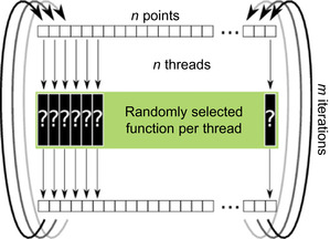 |
| Figure 18.2
Naive parallelizing approach of the Chaos Game. The parallelization is realized by assigning a thread to each data point. Every thread chooses a random function and replaces the point by the computed value. This process is repeated
m
times.
|
Selecting a random function per sample results in a different branch per thread, if the algorithm is implemented on graphics hardware. One needs to consider that these devices execute the same instruction in lockstep within a
warp
of 32 threads. That is, the multiprocessor can execute a single branch at a time, and therefore, diverging branches are executed in serial order.
The random function selection causes very heavy branch divergence as every thread needs to evaluate a different function in the worst case. This results in linear runtime complexity in the number of functions, thus severely restricting the number of functions that can be used in practice, owing to the computational overhead involved.
18.1.1. Iterated Function Systems
As described in
[1]
, an IFS consists of a finite set of affine contractive functions
 The set
 for example forms a Sierpinski triangle with
 where
p
is a vector.
where
p
is a vector.
(18.1)
(18.2)
The associated set
S
is the fixed point of Hutchinsons's recursive set equation
 It is not possible to directly evaluate the set, as the Hutchinson Equation (Eq. 18.3
) describes an infinite recursion. An approximate approach is the Chaos Game
[1]
, which solves the Hutchinson Equation by a Monte Carlo method.
Figure 18.3
shows it in a basic version. The Chaos Game starts by selecting a random point of the bi-unit square
p
= (x
,
y
) with |
x
| ≤ 1, |
y
| ≤ 1 and starts its iterating phase by choosing a random function
f
i
in each iteration and evaluates
p
:=
f
i
(p
). With increasing numbers of calculated iterations,
p
converges closer to the set
[6]
. After a sufficient number of steps, the point can be plotted in every iteration.
It is not possible to directly evaluate the set, as the Hutchinson Equation (Eq. 18.3
) describes an infinite recursion. An approximate approach is the Chaos Game
[1]
, which solves the Hutchinson Equation by a Monte Carlo method.
Figure 18.3
shows it in a basic version. The Chaos Game starts by selecting a random point of the bi-unit square
p
= (x
,
y
) with |
x
| ≤ 1, |
y
| ≤ 1 and starts its iterating phase by choosing a random function
f
i
in each iteration and evaluates
p
:=
f
i
(p
). With increasing numbers of calculated iterations,
p
converges closer to the set
[6]
. After a sufficient number of steps, the point can be plotted in every iteration.
(18.3)
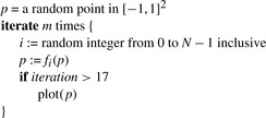 |
| Figure 18.3
The Chaos Game Monte Carlo algorithm. It chooses a random point and starts its iteration phase. Every iteration, a random function
f
i
is selected and evaluated for
p
which is then assigned to
p
.
|
Iterated Function Systems have numerous applications, as outlined in
[3]
, such as graphs of functions, dynamical systems, and brownian motion. Furthermore, this approach could be used in multilayer material simulations in ray tracing. In this chapter, we concentrate on IFS for the simulation of Fractal Flames.
We chose to start with a random point and to select a function at random, even though randomness is not a requirement of the algorithm. The initial point is actually arbitrary; and it will still converge to the set, given that the last iterations contain all possible combinations of functions. As we aim for real-time performance, we can evaluate only a very limited number of iterations, but on a lot of points, exploiting parallelization. Should the resulting fractal be too complicated to achieve subpixel convergence, the random initialization still creates a uniform appearance. This is, especially over the course of some frames, more visually pleasing than deterministic artifacts.
18.1.2. Fractal Flames
Fractal Flames, as described in
[2]
, extend the IFS algorithm by allowing a larger class of functions that can be in the set
F
. The only restriction that is imposed on the functions
f
i
is the contraction on average. These functions can be described by:
 with
P
i
(x
,
y
) = (α
i
x
+
β
i
y
+
γ
i
, δ
i
x
+
ϵ
i
y
+
χ
i
), where
a
i
⋯
g
i
and
α
i
⋯
χ
i
express affine transformations on 2-D points, while
V
j
, so-called
variations
apply nonlinear transformations, which are scaled by the factors
v
ij
. Typically, each function has its own set of up to 20 variations
V
j
. A few variation functions can be found in
Figure 18.4
. An extensive collection of those variations can be found in
[2]
.
with
P
i
(x
,
y
) = (α
i
x
+
β
i
y
+
γ
i
, δ
i
x
+
ϵ
i
y
+
χ
i
), where
a
i
⋯
g
i
and
α
i
⋯
χ
i
express affine transformations on 2-D points, while
V
j
, so-called
variations
apply nonlinear transformations, which are scaled by the factors
v
ij
. Typically, each function has its own set of up to 20 variations
V
j
. A few variation functions can be found in
Figure 18.4
. An extensive collection of those variations can be found in
[2]
.
(18.4)
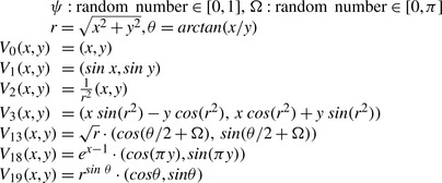 |
| Figure 18.4
A few selected variation functions. Ω and
ψ
are new random numbers in each evaluation of the variation function.
|
Every function is assigned a weight
w
i
that controls the probability that
f
i
is chosen in a Chaos Game iteration. This parameter controls the influence of a function in the computed image. Furthermore, a color
c
i
∈ [0, 1] is assigned. Every point has a third component that holds the current color
c
, which is updated by
c
:= (c
+
c
i
)/2 in each iteration and is finally mapped into the output color space.
The computed points are visualized by creating a colored histogram. Because the computed histogram has a very high dynamic range, a tone-mapping operator is applied.
18.2. Core Technology
In order to remove branch divergence, we replace the randomness of the function selection by randomized data access. This way, instructions can be optimally and statically assigned to threads.
Warps are assigned to a fixed function and every thread randomly selects a data point in each iteration. This selection is realized by a random bijective function mapping between the data and the thread indices. A fixed set of precomputed permutations is used, as they don't depend on dynamic data and may be cyclic, for it doesn't matter if the generated images repeat after a few rendered frames.
Every thread calculates its assigned function and indirectly accesses the data array by its permuted index. It then evaluates the function and writes back the result. A new permutation is picked in each iteration.
Figure 18.5
shows the iteration scheme.
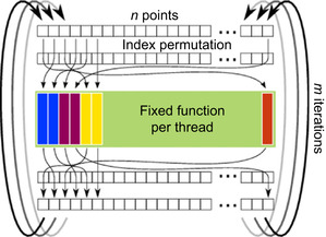 |
| Figure 18.5
Optimized parallel algorithm. Instead of indexing directly into the data array as in
Figure 18.2
, the data is shuffled randomly in every iteration. This allows one to statically assign threads to functions and thereby remove the branch divergence.
|
18.3. Implementation
The optimized algorithm and the divergent approach have been implemented to benchmark both of them. The implementation uses CUDA to be able to tightly control the thread execution that would not have been possible with traditional shading languages.
All variation functions have been implemented in a large switch statement. A struct containing variation indices and the scalar factor is stored in the constant memory. To evaluate a function
f
i
, a loop
over all those indices is performed that is used to index in the switch statement. The results are summed up according to
Eq. 18.4
.
18.3.1. The Three Phases
The optimized Chaos Game algorithm requires synchronization across all threads and blocks after each iteration because the data gets shuffled across all threads. Because of CUDA's lack of such a synchronization instruction, the Chaos Game had to be split into three kernels to achieve synchronization by multiple kernel executions (see
Figure 18.6
and
Figure 18.7
).
 |
| Figure 18.6
Illustration of the pseudo-code listing in
Figure 18.7
. The left three large boxes are the kernels (init, warm-up, generate), the last representing rendering in OpenGL. Memory access patterns are indicated by the gray lines. On the left,
h
indicates the Hammersley point set as the input.
|
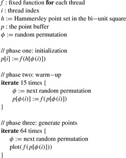 |
| Figure 18.7
The three phases of the GPU version of the Chaos Game. First,
p
is initialized by transforming the Hammersley points by one function evaluation. Second, the warm-up phase assures that the points
p
are sufficiently close to the fractal. Finally, the point set is transformed 64 times more. In this last phase, the transformed points are displayed, but not written back to
p
.
|
The initialization kernel performs one iteration of the Chaos Game on the randomly permuted Hammersley point set. The warm-up kernel performs one Chaos Game iteration and is called multiple times until the output data points converged to the fractal. The last kernel generates a larger set of points by randomly transforming each of the previously generated points 64 times, producing 64 independent samples for each input sample. The generated points are recorded in a vertex buffer object (VBO), which is then passed to the rendering stage. From those kernels, the point-generation kernel takes by far the most computation time. Those runtimes on a GTX280 are 34.80μs init, 43.12μs warm-up, and 1660.59μs generate points. The init kernel occupies 1.5% of the total Chaos Game runtime; the warm-up kernel is called 15 times and thus takes 27.6%, whereas the point-generation kernel takes 70.9%.
18.3.2. Memory-Access Patterns
The point-generation kernel needs to select a point from the point buffer multiple times, calculate one iteration, and write the result into the VBO. As the input point array does not change, texture caching can be used. The effect of this optimization is a 6.9% speed improvement for the 9500GT and 18% for the GTX280. The access pattern is pretty bad for the texture-caching mechanisms of a GPU because it completely lacks locality. Because the memory consumption of the samples is approximately 200 kB,
the cache of a GPU seems to be big enough to hold a large number of samples; therefore, this method yields a major performance improvement. Benchmarks have been conducted to measure the effect of the number of samples on the texture caching. As shown in
Figure 18.8
, the number of threads — and therefore the number of samples in the texture cache — doesn't have a huge impact: the runtime stays
constant up to 2
12
threads and then increases linearly with the number of threads; the cached version is constantly faster.
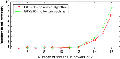 |
| Figure 18.8
Runtime on the GTX280 in dependence of number of running threads. Each thread generates 64 samples. The runtime stays almost constant to 2
12
threads and subsequently increases linearly with the number of threads.
|
Note that only the warm-up kernel has a completely random memory-access pattern during read and write. It needs to randomly access the point array to read a point for the iteration and to write out its result. To avoid race conditions on write accesses, either data has to be written back to the position the point was read from, or else a second array storing points is needed. The former approach involves random reads and writes, whereas the latter one has higher memory use. The initialization kernel needs to randomly select a starting point, but it can write the iterated points in a coalesced manner. Because of its low runtime, there is no need to optimize it further.
18.3.3. Rendering
The generated points are rendered as a tone-mapped histogram using OpenGL. This step consumes approximately 70% of the total time, depending on the particular view.
The 1-D color component needs to be mapped into the RGBA(red, green, blue, alpha) representation. This is done by a 1-D texture look-up in a shader. To create the colored histogram, the points are rendered using the OpenGL point primitive and using an additive blending mode. This yields brighter spots where multiple points are drawn in the same pixel. To cope with the large range of values, a floating-point buffer is employed. The resulting histogram is then tone mapped and gamma corrected, because the range between dark and bright pixel values is very high. For the sake of simplicity and efficiency, we use
L
′ =
L
/(L
+ 1) to calculate the new pixel lightness
L
′ from the input lightness
L
, but more sophisticated operators are possible
[2]
.
Monte Carlo-generated images are typically quite noisy. This is especially true for the real-time implementation of Fractal Flames because only a limited number of samples can be calculated in the given time frame. Using temporal antialiasing smoothes out the noise by blending between the actual frame and the previously rendered ones. This is implemented by using frame buffer objects and it increases the image quality significantly.
Some static data is needed during runtime; this data is calculated by the host during program start-up. A set of Hammersley Points
[4]
is used as the starting-point pattern to ensure a stratified distribution, which increases the quality of the generated pictures. The presorting algorithm needs permutations that are generated by creating multiple arrays containing the array index and a random number calculated by the Mersenne Twister
[5]
. These arrays are then sorted by the random numbers, which can be discarded afterwards. The resulting set of permutations is uploaded onto the device. Since some of the implemented functions need random numbers, a set of random numbers also is created and uploaded onto the device. All of this generated data is never changed during runtime.
In the runtime phase, it is necessary to specify various parameters that characterize the fractal. Every function needs to be evaluated in
p
(f
i
) ⋅
num_threads
threads, where
p
(f
i
) is the user-specified probability that function
f
i
is chosen in the Chaos Game. The number of functions is small compared to the number of threads, and therefore, it doesn't matter if this mapping is done in warp size granularity instead of thread granularity. Each thread is mapped to a function by an index array that is compressed into a prefix sum. A thread can find out which function it has to evaluate by performing a binary search on this array. This search does not introduce a performance penalty in our experiments, but reduces the memory requirements significantly. The parameters and the prefix sum are accumulated in a struct that is uploaded into the constant memory each frame.
18.4. Final Evaluation
The naive parallel implementation degenerates to an
O
(n
) algorithm in the number of functions on graphics hardware due to the branch divergence issues. The proposed algorithm turns the function evaluation in the naive Chaos Game algorithm to an
O
(1) solution. This is shown in
Figure 18.9
and
Figure 18.10
, where the optimized algorithm is benchmarked against the naive parallel implementation on a 9500GT and a 280GTX, respectively. In the benchmark, 20 randomly selected variation functions
V
j
were used in each
f
i
. The evaluation time of the optimized algorithm stays constant, whereas the naive solution increasingly suffers from branch divergence issues. When the CUDA profiler is employed, the branch divergence can be measured. The amount of branch divergence with 20 activated functions is at 23.54% for the divergent approach, whereas the optimized algorithm shows branch divergence only inside the function evaluation (0.05%).
 |
| Figure 18.9
Runtime comparison between divergent and optimized Chaos Game on a 9500GT in dependence on the number of activated functions. The divergent implementation shows linearly increasing runtime in the number of activated functions, while the optimized algorithm shows constant runtime. The optimized version beats the divergent solution when eight or more functions are activated.
|
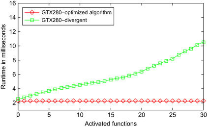 |
| Figure 18.10
A runtime comparison between divergent and optimized Chaos Game on a GTX280 in dependence on the number of activated functions. The performance characteristics are the same as with the 9500GT shown in
Figure 18.9
, with a smoother increase in the divergent graph. The optimized version is always faster.
|
The optimization doesn't come without cost, though. The algorithm basically trades branch divergence for completely random memory-access patterns. As the benchmark shows, GPUs handle this surprisingly well. Different GPUs have been benchmarked to show that this behavior isn't restricted to high-end GPUs (the speed impact of permuted read-and-write access versus completely linear operations was 3.1% for the 9500GT and 5.3% for the 280GTX).
In
Figure 18.11
, it is shown that the Chaos Game runtime is not monotonically decreasing with increasing block size. The best runtime is achieved with 64 threads per block. It is not entirely clear from where this behavior arises, but it may be that the scheduler has a higher flexibility with smaller block sizes.
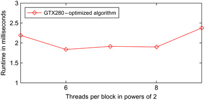 |
| Figure 18.11
Runtime changing with increasing block size and constant number of threads. The fastest configuration is a block size of 2
6
.
|
In our implementations, the occupancy as reported by the CUDA profiler is 0.25. This is due to high-register usage of the function evaluation code. Enforcing a lower-register usage at compile time increases the occupancy to 1.0 but reduces the performance by 51.3%.
We additionally implemented a CPU version to verify the benefits of using graphics hardware. Benchmarks have shown that a GTX285 is able to perform the Chaos Game iterations, without the rendering, at about 60 times faster than a single-core Opteron CPU clocked at 2.8 GHz (240 Hz vs. 3.7 Hz).
18.5. Conclusion
A presorting approach has been presented that completely eliminates branch divergence in Monte Carlo algorithms that use random-function selection and evaluation. Furthermore, it was shown that the approach is sufficiently fast for real-time rendering at high-frame rates, while it is necessary to keep an eye on the imposed performance penalty owing to high-memory bandwidth costs.
The optimized approach allows us to change all parameters in real time and to observe their effects; it thus can effectively help in getting an understanding of Iterated Function Systems. This also makes it possible to use the Fractal Flames algorithm in live performances by changing the parameters in real time, conducting interactive animations.
References
[1]
M. Barnsley,
Fractals Everywhere: The First Course in Deterministic Fractal Geometry
. (1988
)
Academic Press
,
Boston
.
[2]
S. Draves, E. Reckase,
The fractal flame algorithm
(2008
)
;
http://flam3.com/flame_draves.pdf
.
[3]
K. Falconer, K.J. Falconer,
Fractal Geometry: Mathematical Foundations and Applications
. (1990
)
Wiley
,
New York
;
(Chapters 9–18)
.
[4]
C. Lemieux,
Monte Carlo and Quasi-Monte Carlo sampling
. (2009
)
Springer Verlag
,
Berlin
.
[5]
M. Matsumoto, T. Nishimura,
Mersenne twister: a 623-dimensionally equidistributed uniform pseudo-random number generator
,
ACM Trans. Model. Comput. Simul. (TOMACS)
8
(1
) (1998
)
3
–
30
.
[6]
B. Silverman,
Density Estimation for Statistics and Data Analysis
. (1998
)
Chapman & Hall/CRC
,
London
.
..................Content has been hidden....................
You can't read the all page of ebook, please click here login for view all page.