
Chapter 34. Experiences on Image and Video Processing with CUDA and OpenCL
Alptekin Temizel, Tugba Halici, Berker Logoglu, Tugba Taskaya Temizel, Fatih Omruuzun and Ersin Karaman
This chapter will be helpful to those, in particular academicians and professionals, who work with compute- and data-intensive image and video processing algorithms.
The chapter addresses the technical challenges and experiences associated with the domain-related algorithms implemented on GPU architectures specifically by using CUDA and OpenCL with an emphasis on real-time issues and optimization. We present a series of implementations on background subtraction and correlation algorithms, each of which addresses different aspects of GPU programming issues, including I/O operations, coalesced memory use, and kernel granularity. The experiments show that effective consideration of such design issues improves the performance of the algorithms significantly.
34.1. Introduction, Problem Statement, and Background
The importance of GPUs has recently been recognized for general-purpose applications such as video and image processing algorithms. An increasing number of studies show substantial performance gains with their GPU-adapted implementations. Video and image processing algorithms, in particular, real-time video surveillance applications, have gained ground owing to the growing need to ensure public security worldwide. They have now become viable to realize in high-camera-number cases, thanks to GPUs.
In this chapter, we implement two image and video processing applications on the CPU and the GPU to compare their effectiveness. As a video processing application, adaptive background subtraction, and as an image processing application, Pearson's correlation algorithms have been implemented.
Although there are studies showing parallel implementations for a myriad of image and video processing algorithms on GPUs, their performance evaluations are limited by specific platforms and computing architectures and without any concern for real-time issues. Moreover, they fail to guide the researchers and developers in terms of platform and computing architecture capabilities. For example, an algorithm is implemented using CUDA, and the performance comparison is often carried out between the CPU and the GPU mostly on a specific platform.
This study aims to guide users in implementing GPU-based algorithms using CUDA and OpenCL architectures by providing practical suggestions. In addition, we compare these two architectures to demonstrate their advantages over each other, in particular, for video and image processing applications.
In this study, we focus on two widely used algorithms in computer vision and video processing: adaptive background subtraction and Pearson correlation.
The first one is an adaptive background subtraction algorithm that can be used to identify moving or newly emerging objects from subsequent video frames. This information can then be used to enable tracking and deducting higher-level information that is valuable for automated detection of suspicious events in real time (see
Figure 34.1
). We selected the algorithm described in
[1]
because this cost-effective method is easy to implement and produces effective results. The algorithm is embarrassingly parallel in nature because the same independent operation is applied to each pixel in a frame.
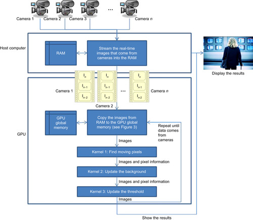 |
| Figure 34.1
The flowchart of the background subtraction algorithm.
|
We have considered the following domain-specific constraints regarding a typical video surveillance application in our study. In order to achieve real-time processing with PAL (Phase Alternating Line) format videos, the number of frames processed per second (fps) was determined as 25. To perform this task in real time, we note that images from all cameras should be processed in 40ms, prior to the arrival of the subsequent frames. The maximum number of cameras that can be supported in the GPU architecture is obtained by calculating the number of video frames that can be processed simultaneously in real time with this constraint.
Real-time processing is of great importance, particularly in the security domain. Until recently, officers have been able to deal with tracking suspicious cases in real time. However, a high number of cameras, combined with an increase in security risks in crowded public places, such as in airports, underground stations or terminals, and town squares, necessitate the automation of surveillance process in real time because it is no longer possible to carry out this process manually. Real-time processing is also required in other video applications, such as automated video content analysis and robotics.
The second algorithm is Pearson correlation, which is used to measure the similarity of two images. The application areas of the algorithm are numerous. For example, the algorithm may aid the security officers to compare registered cartridge cases in a database with one obtained in a crime scene. This computation can be carried out in parallel for
N
number of images independent of each other. To achieve good performance, however, it is important to avoid reaccessing the compared image many times from the global memory and to keep the interim correlation results in the local memory to have a better performance.
34.2.1. Background Subtraction
The algorithm consists of three main stages:
• Finding moving pixels
• Updating the background
• Updating thresholds
With each new image, moving pixels are found, and
B
n
and
T
n
are updated according to the following rules.
Finding Moving Pixels
(34.1)
Updating the Background
Background is updated with each new image, according to the following equation:
 If the pixel is moving, background is updated using a time constant
α
; otherwise, it is kept the same.
α
, (0 <
α
< 1), determines how the new information updates older observations. An
α
closer to 1 means that the older observations have higher weight and the background is updated more slowly.
If the pixel is moving, background is updated using a time constant
α
; otherwise, it is kept the same.
α
, (0 <
α
< 1), determines how the new information updates older observations. An
α
closer to 1 means that the older observations have higher weight and the background is updated more slowly.
(34.2)
Threshold is updated with each new image according to the following equation:
 Similar to the background update, if the pixel is moving, threshold is updated using the time constant
α
; otherwise, it is kept the same. The threshold
c
is a real number greater than one, analogous to the local temporal standard deviation of the intensity. In our experiments we used
c
= 3 and
α
= 0.92.
Similar to the background update, if the pixel is moving, threshold is updated using the time constant
α
; otherwise, it is kept the same. The threshold
c
is a real number greater than one, analogous to the local temporal standard deviation of the intensity. In our experiments we used
c
= 3 and
α
= 0.92.
(34.3)
Some examples from the background subtraction algorithm with the i-Lids dataset
[2]
are shown in
Figure 34.2
.
 |
| Figure 34.2
Images illustrating the background subtraction algorithm. The original image
In
(top left), extracted background image
Bn
(top right), moving pixels (bottom left), threshold image
Tn
(bottom right).
|
Correlation is a technique for measuring the degree of relationship between two variables. It is used in a broad range of disciplines, including image/video processing and pattern recognition. The relationship between the variables is obtained by the calculation of coefficients of correlation. There are a number of different coefficients, including Kendall's tau correlation coefficient and Spearman's rho correlation coefficient, but the most popular and widely used one is that of Pearson's correlation coefficient (PMCC) aka sample correlation coefficient. It takes values between [−1, 1] where 1, 0 and −1 indicate a perfect match, that is, no correlation and perfect negative correlation, respectively.
PMCC is defined as the covariance of the variables that are to be compared, divided by their standard deviations:


(34.4)
(34.5)
(34.6)
34.3. Key Insights from Implementation and Evaluation
In this section, we discuss the two algorithms’ performances in detail.
Table 34.1
shows the parameters used in the experiments. Four different video sizes and three different GPUs have been used.
We implemented the algorithms on the GPU using OpenCL and CUDA and parallelized the algorithms on the CPU using OpenMP. OpenMP implementations were implemented using Visual Studio 2008.
34.3.1. Case Study 1: Real-Time Video Background Subtraction
In this case study, we implemented the background subtraction algorithm
[1]
that was explained in the previous sections on CPUs and GPUs. For the single-kernel case, all three steps of the algorithm are integrated in a single kernel. For the multikernel case, three separate kernels consisting of individual steps — namely, finding moving pixels, updating the background, and updating thresholds — are used. These three kernels are then run successively. In the experiments, we use four different image sizes: 160 × 120, 320 × 240, 640 × 480, and 720 × 576. The number of threads and block size are set to 64 and 512, respectively.
The main components of the algorithm (corresponding to
(34.1)
(34.2)
and
(34.3)
) are illustrated in
Example 34.1
Example 34.2
and
Example 34.3
with CUDA codes. Threshold pixels (Tn) are set to 127, and background pixels (Bn) are set to 0 at initialization.
Finding the moving pixels
1 __global__ void FindMovingPixels(unsigned char *In, unsigned char*In_1, unsigned char *In_2, unsigned char *Tn, __global char *MovingPixelMap)
2 {
3
long int index = blockDim.x * blockIdx.x + threadIdx.x;
4
if(abs(In[i] − In_1[i]) > Tn[i] && abs(In[i] − In_2[i]) > Tn[i]) {
5
MovingPixelMap[i] = 255;
6
}
7
else {
8
MovingPixelMap[i] = 0;
9
}
10 }
Updating the background
1 __global__ void updateBackgroundImage(unsigned char *In, unsigned char * MovingPixelMap, unsigned char *Bn)
2
{
3
long int index = blockDim.x * blockIdx.x + threadIdx.x;
4
if(MovingPixelMap [i] == 0) {
5
Bn[i]=0.92*Bn[i] + 0.08*In[i];
6
}
7
}
Updating the threshold
1 __global__ void updateThresholdImage(__global const char *In, __global char *Tn, __global char *MovingPixelMap, __global char *Bn)
3
long int index = blockDim.x * blockIdx.x + threadIdx.x;
4
int minTh = 20;
5
float th = 0.92* Tn[i] + 0.24 *(In[i] − Bn[i]);
6
if(moving_pixel_map[i]==0) {
7
if(th > minTh) {
8
Tn[i] = th;
9
}
10
else {
11
Tn[i] = minTh;
12
}
13
}
14
}
Figure 34.3
and
Example 34.4
show the memory handling where redundant copies are avoided and three image buffers are used throughout the entire lifetime of the algorithm. With each new image, pointers are swapped, as shown in
Example 34.4
and the new image is copied from the host to the GPU memory (the seventh line, which is shown in the light gray boxes in
Figure 34.3
). In performance calculations where I/O operation is excluded, this line is not taken into account.
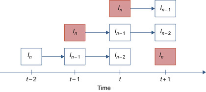 |
| Figure 34.3
The relationship between current and former frames. Frames
I
n
and
I
n
− 1
at time
t
−
1
are copied into
I
n
− 1
and
I
n
− 2
at time
t
, respectively. New
I
n
value is copied from the host computer's memory.
|
Swapping buffers
1 void SwapBuffers()
2 {
3
Unsigned char *tempMem;
4
tempMem = GPU_In_2;
5
GPU_In_1 = GPU_In;
6
GPU_In = tempMem;
7
CopyFromHostToDevice(GPU_In,CPU_In,sizeof(In));
8)
The images reside in global memory. We did not consider using shared memory because each pixel is accessed only once. Also, coalescing of the image data is not an issue for this algorithm because threads work on subsequent pixels.
In order to measure the performances, we calculate the maximum number of cameras that can be processed in real time. We assume a real-time constraint of 25 frames per second; hence, we calculate the number of images that can be processed in 40ms to find out the number of cameras supported in real time.
34.3.2. Experiment 1: Single Kernel Only: Performance Gains with and without I/O Operations
In this experiment, we aim to measure how much speedup we get using various image resolutions on different GPU architectures compared with the CPU. We first find the maximum number of cameras supported with different image resolutions on Intel i7 920 architecture using OpenMP to utilize all four cores of this processor. Then, we measure the number of supported cameras on different GPU architectures. The performance gain is calculated by dividing the GPU results to the CPU results.
As can be seen from
Figure 34.4
, GPU2 (GTX 285) has achieved the highest performance, whereas GPU3 (9800 GT) has performed the lowest. CUDA is approximately two to three times faster than
OpenCL for all cases.
Figure 34.4
and
Figure 34.5
show the performance gain ratios for cases when I/O is not included and when I/O is included, respectively.
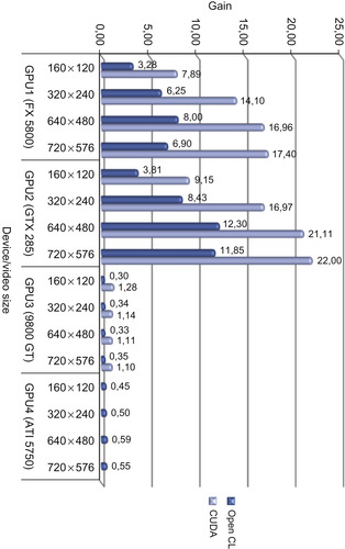 |
| Figure 34.4
Performance gain ratio of various GPUs vs. OpenMP CPU (Intel i7 920) implementation (I/O not included).
|
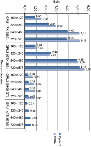 |
| Figure 34.5
Performance gain ratio of various GPUs vs. OpenMP CPU (Intel i7 920) implementation (I/O included).
|
For the case where I/O time is included, even though CUDA has still higher performance, the gain decreases, and the performance gets closer to the OpenCL version. This is owing to the I/O operation time dominating over the processing time and making the effect of processing time less significant for the overall results. Although up to a 22x increase could be observed when I/O time is not included, this drops to 5.6x when the I/O time is included. This drop could be remedied to a degree by overlapping the memory copy operations with the processing, as will be described later.
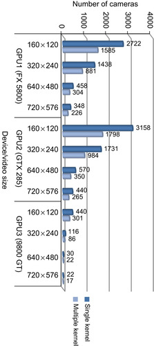
An important parameter is the maximum number of cameras that can be supported for real-time operation.
Figure 34.5
and
Figure 34.6
show the results for cases when an I/O was not included and when an I/O was included, respectively. These experiments have been conducted with a single-kernel version to get the best performance for all devices used in the experiment. Even though the cases when the I/O was not included give the theoretically highest performance, it is not realistic because the data needs to be copied from the host to the device memory. In order to make a fair comparison, the measurements should include the time spent for data transfer from the host to the device.
 |
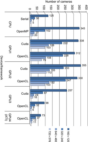
| Figure 34.6
Maximum number of cameras that can be supported for real-time operation using CPU and GPUs (I/O not included).
|
As can be observed from
Figure 34.6
and
Figure 34.7
, the I/O operation during which the image data are copied from the host to the device have a significantly adverse effect on performance. Hence, we implemented an asynchronous version in which the memory copy and processing operations are overlapped (i.e., an image is processed while the next image is copied from the host simultaneously). This asynchronous version is shown in
Example 34.5
. Here, the kernel operation
cuda_process_frames()
and
memory copy
cudaMemcpyAsync()
are given two different stream parameters
stream1
and
stream2
. Each stream runs asynchronously independent of other streams.
 |
| Figure 34.7
Maximum number of cameras that can be supported for real-time operation using CPU and GPUs (I/O included).
|
Asynchronous version
1 cudaStream_t stream1, stream2;
2 cudaStreamCreate(&stream1);
3 cudaStreamCreate(&stream2);
4 cuda_process_frames<<<dimGrid,dimBlock,stream1>>>(In_D,In_1_D,In_2_D,Th_D,Bn_D, moving_pixel_map_D,framesize);
5 cudaMemcpyAsync(In_D_async,In,framesize,cudaMemcpyHostToDevice,stream2);
6 cudaThreadSynchronize();
7 char *tmp = In_D;
8 In_D = In_D_async;
9 In_D_async = tmp;
The results for this implementation are illustrated in
Figure 34.8
and
Figure 34.9
. It has been observed that up to 9x performance gain could be achieved for 720 × 576 images compared with the OpenMP CPU implementation. It has to be noted that this gain drops when the image sizes get smaller.
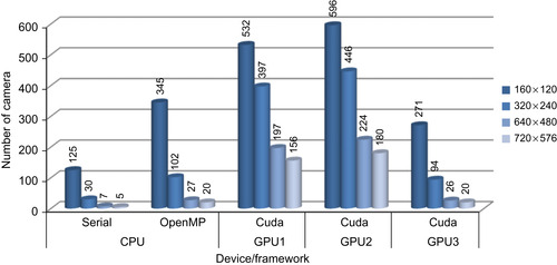 |
| Figure 34.8
Maximum number of cameras that can be supported for real-time operation using CPU and GPUs (I/O included, asynchronous operation).
|
 |
| Figure 34.9
Performance gain ratio of various GPUs vs. OpenMP CPU (Intel i7 920) implementations (asynchronous).
|
34.3.3.
Experiment 2: Single Kernel vs. Three Kernels: Performance Gains with and without I/O Operations
We have implemented a single-kernel version where all operations are gathered in a single kernel and a multiple-kernel version where the three main steps of the algorithms are implemented in three different kernels that are called subsequently. The total number of cameras that can be supported in this case is shown in
Figure 34.10
. As illustrated in this figure, increasing the number of kernels brings a significant overhead where the performance decreases as much as 43%. This is due to each kernel accessing the memory independently and hence requiring multiple accesses to the same data. On the other hand, in the single-kernel case, data is fetched once. It is also interesting to note that OpenCL suffers more heavily compared with CUDA. This performance difference is less when I/O time is included.
 |
| Figure 34.10
Comparison of the maximum number of cameras that can be supported for real-time operation using single-kernel and multiple-kernel GPU implementations.
|
As a general rule, it is suggested that the number of kernels are kept at a minimum to avoid the performance penalty owing to multiple accesses to the memory and overhead in initiating kernel calls when the runtime of the kernel is relatively short.
34.3.4. Experiment 3: Single Kernel Only: Performance Gains with Serial I/O and Asynchronous I/O
Because the serial I/O case doesn't reflect real performance gains, and serial I/O is not the best method for achieving the best performance, an asynchronous version has been implemented, as illustrated in
Example 34.5
. The comparison of these versions is shown in
Figure 34.11
(serial I/O vs. asynchronous I/O 8-bit reads).
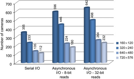 |
| Figure 34.11
A comparison of the maximum number of cameras that can be supported for real-time operation using serial I/O, asynchronous I/O- 8-bit reads, and asynchronous I/O- 32-bit reads using GPU2.
|
The results show that a much higher number of cameras could be processed using asynchronous calls compared with using serial I/O. For example, with asynchronous calls, 68%, 91%, 66%, and 61% more cameras could be processed for 160 × 120, 320 × 240, 640 × 480, and 720 × 576 resolutions, respectively.
Although the performance gains were significant, they were not the same for all image sizes. For example, the highest gain was observed for images with 320 × 240 resolution. This is due to a lesser difference between the time spent on I/O operations required for copying images from the host computer's memory to the GPU's global memory and the processing time for background subtraction on GPUs as verified using Visual Profiler. If one of the operations takes more time than the other, latency will occur. For example, if I/O operations take more time than the computations, the kernel will wait for image transfer or vice versa.
As a result, I/O operations are essential parts of the applications, and they cannot be avoided in measuring performances. Asynchronous calls should always be preferred if the application logic is suitable.
34.3.5. Experiment 4: Reading 8 Bits vs. Reading 32 Bits from the Global Memory
In the previous experiments, we used
unsigned char
to access 8-bit image data from the global memory. Memory reads in GT200 are done for half-warps of 16 threads, and reads are done for 32, 64, or 128 bytes. In the previous cases, as each thread reads a byte, 16 bytes are read. For better utilization of global memory bandwidth, these reads have to be 32, 64, or 128 bytes. In the context of the problem in hand, this can be achieved by first reading 4
chars
per thread and then processing each
char,
which results in 16 * 4 = 64 bytes reads for each half-warp.
Example 34.6
demonstrates reading of data in 32-bit chunks processing 4- × 8-bit elements by each thread. Note that in this case only the current image In and the background Bn are loaded from the global memory, and Bn is written back to the global memory. For a complete implementation all the other images In_1, In_2, Bn, Tn, and MovingPixelMap should also be loaded in a similar fashion.
Steps for 32-bit access to the global memory
1 __global__ void processImage(unsigned int *In, unsigned int *Bn) {
2 long int index = blockIdx.x * N + threadIdx.x * 4;
3 unsigned int packedIn = In[index]; // Read an int from the global memory
4 unsigned int packedBn = Bn[index]; // Read an int from the global memory
5 unsigned int bnout = 0;
6 for(int i=0; i < 4; i++) {
7
unsigned int in = (packedIn & 0x0ffu); // read a char from packed data
8
int outdata = …;//Process the data here, each thread processes 4-chars
9
bnout += ((unsigned int)(outdata)) << (i * 8); // pack the output
10
packedIn >>= 8; packedBn >>= 8;// Move to the next char
11
}
12 Bn[index] = bnout; // Copy the result back to the global memory
13 }
The results show that higher-number cameras could be processed using 32-bit reads, as shown in
Figure 34.11
(asynchronous I/O 8-bit reads vs. asynchronous I/O 32-bit reads). Compared with 8-bit reads, 8%, 12%, 18%, and 29% more cameras could be processed for 160 × 120, 320 × 240, 640 × 480, and 720 × 576 resolutions, respectively.
In this case study, we implement the Pearson correlation algorithm that was explained in previous sections on CPUs and GPUs. We have implemented two different approaches that differ on the memory types used for the calculation of
ρ
x, y
, the Pearson's correlation coefficient. The first approach is using only the global memory of the GPU, whereas the second utilizes the shared memory along with the global memory.
The GPU implementation of the algorithm significantly differs in parallelization from the background subtraction in the way that in this algorithm each worker cannot be assigned to each pixel of the image because the algorithm is composed of summations. The jobs are rather chosen as the individual image frames to be able to fully utilize the GPU. But it should be noted that this yields two constraints:
Keeping the aforementioned constraints in mind, we diagramed the flowchart of the calculation of Pearson's correlation coefficients in
Figure 34.12
. The flowchart is valid for the both approaches that are utilized.
• A high number of images are needed for high-GPU utilization.
• The images to be compared should be available on the GPU memory.
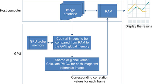 |
| Figure 34.12
A flowchart of the calculation of Pearson's correlation coefficients.
|
34.3.7. Experiment 1: Global Memory Only
As mentioned before, the first approach that uses only the global memory of the GPU is rather straightforward; the given one-pass version for the PMCC formula is directly implemented. Example kernel
code is very similar to the one given for the shared-memory version in
Example 34.6
; thus, the global memory version is not given to avoid duplication.
Experiments have been carried out for four different image sizes: 160 × 120, 320 × 240, 640 × 480, and 720 × 576. The approach is implemented using OpenCL and CUDA. The corresponding results for the comparison of 1024 images are shown in
Figure 34.13
. As seen, once again CUDA performs better than OpenCL at all times. Note that the ATI results are only given for 160 × 120 and 320 × 240 image sizes because the OpenCL implementation has a memory allocation limit and 1024 images of 640 × 480 exceeds this limit.
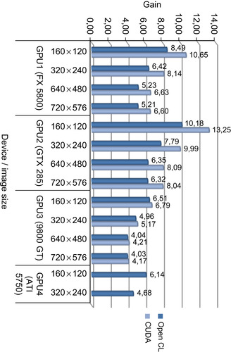 |
| Figure 34.13
Performance gain of OpenCL and CUDA implementations over an OpenMP implementation on the CPU.
|
34.3.8. Experiment 2: Global Memory + Shared Memory with Coalesced Memory Access
One downside of the first approach is that every image to be compared accesses to the same memory space because they are all compared with the same reference image. The same memory that is written in global memory is read over and over again. An approach to overcome this inefficiency is using shared memory spaces that are much faster. The steps of the algorithm can be explained as follows:
1. Occupy a block of shared memory.
2. Calculate how many passes are required to process all the pixels in an image by dividing pixel number by the chosen shared memory block size.
3.
For each pass, first load a block of pixel values of reference image from global to shared memory. Calculate each element
 in
Equation 34.6
within the block using the values in the shared memory when needed. Note that the elements are added up in each step on top of previously calculated values.
in
Equation 34.6
within the block using the values in the shared memory when needed. Note that the elements are added up in each step on top of previously calculated values.
4. At the end of the passes, we end up with calculated elements; thus, just putting the values in
Equation 34.3
, we obtain the correlation coefficient.
The corresponding CUDA kernel for the explained algorithm is given in
Example 34.7
.
PMCC calculation using shared memory — CUDA implementation
1 __global__ void cudaPMCC(float *GPUcorrVal, unsigned char *GPUhostImg, unsigned char *GPUsampleImg, int ImageWidth, int ImageHeight, int GPUimgNumber){
2 int index = blockDim.x * blockIdx.x + threadIdx.x;
3 if(index < GPUimgNumber) {
4 float sum1=0.0f, sqrSum1=0.0f, sum2=0.0f, sqrSum2=0.0f, prodSum=0.0f;
5
__shared__ unsigned char temp[blockDim];
6
int BLOCK_LENGTH = blockDim;
7
int shotCount = (ImageWidth*ImageHeight + BLOCK_LENGTH −1)/BLOCK_LENGTH;
8
for(int shotIndex = 0; shotIndex < shotCount; shotIndex += 1) {
9
int shotBegin = shotIndex * BLOCK_LENGTH;
10
int shotEnd = min(shotBegin + BLOCK_LENGTH, ImageWidth*ImageHeight);
11
int shotLength = shotEnd - shotBegin;
12
int shotRef = shotBegin + threadIdx.x;
13
temp[threadIdx.x] = (unsigned char)GPUhostImg[shotRef];
14
__syncthreads();
15
for(int i=0;i<shotLength;i++) {
16
float val1 = temp[i];
17
float val2 = GPUsampleImg[(shotBegin+i)*GPUimgNumber + index];
18
sum1 += val1;
19
sqrSum1 += val1*val1;
20
sum2 += val2;
21
sqrSum2 += val2*val2;
22
prodSum += val1*val2;
23
}
24
}
25 GPUcorrVal[index] = 0;
26 float count = ImageWidth*ImageHeight;
27 float variance1 = (count*sqrSum1) − (sum1*sum1);
28 float variance2 = (count*sqrSum2) − (sum2*sum2);
29 float covariance = (count*prodSum) − (sum1*sum2);
30 float energySqr = variance1*variance2;
31 if(energySqr > 0)
32 GPUcorrVal[index] = covariance/sqrt(energySqr);
33 }
34 }
One more important issue that is considered in our study is the memory access. The images to be processed are arranged for coalesced memory access for optimal performance. The details of the memory arrangement are given in
Figure 34.14
.
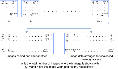 |
| Figure 34.14
Memory arrangement for coalesced memory access.
|
Where
N
is the total number of images where
n
th image is shown with
I
n
,
w
and
h
are the image width and height, respectively.
The performance gains obtained by utilizing shared memory (vs. first approach) and coalesced access (vs. first approach) for images of size 320 × 240 are given in
Figure 34.15
. The tests are conducted for a comparison of 1024 images, as done in the first approach's experiment. It is observed that coalesced memory arrangement boosts the performance up to 4.34 times. Further performance improvements could be obtained by using shared memory in addition to using this approach.
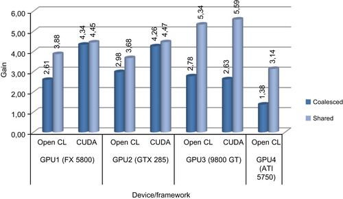 |
| Figure 34.15
Performance gain of using shared-memory and coalesced-memory arrangements for 320 × 240 image sizes.
|
34.3.9. Experiment 3: Effect of Increasing the Number of Images
This experiment's goal is to see the effect of the number of images on the performance gain. Four different image numbers are used for experiments: 1024, 2048, 4096, and 8192.
Figure 34.16
shows the performance gains obtained for images of size 160 × 120 for both OpenCL and CUDA implementations using both shared-memory and coalesced-memory arrangements compared with OpenMP CPU implementation.
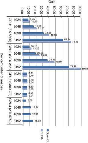 |
| Figure 34.16
Performance gain for increasing image number over OpenMP implementation on the CPU for 160 × 120 image sizes.
|
As seen from
Figure 34.16
, with the increasing number of images, the performance gain increases for GPUs with a high number of multicores because utilization increases for those GPUs. As a result of efficiency, comparison of 8192 images of size 320 × 240 was performed 89.84 times faster than the OpenMP CPU implementation.
In this chapter, we have compared the performance of background subtraction and correlation algorithms on the GPU using CUDA and OpenCL, and on the CPU by using OpenMP. We then discussed the results. We showed that up to 11.6x and 89.8x increases in performance could be achieved for these algorithms, respectively, compared with their CPU implementations. To get the most out of GPU-based computing, several issues need to be taken into consideration during the implementation of a parallelizable image and video processing applications on the GPU.
Because the memory I/O operations affect the performance of the application significantly, they have to be optimized, and data decomposition should be carried out with caution. Working with larger images (720 × 576) rather than smaller images (160 × 120) results in better performance gain. Asynchronous memory copying should be implemented wherever possible to overlap processing and data transfer. Algorithms need to be designed to prevent redundant memory copy operations. In certain video processing applications, preceding video frames might be required. So if one manages the image buffer using pointer swaps, rather than making copy operations, redundancy could be avoided.
Besides implementing efficient memory access between the CPU and GPU memories, we found that efficient GPU memory access is also vital for performance. Coalesced-memory access has to be preferred, and one should arrange the data for coalesced access whenever possible. For example, for the correlation algorithm, the image database could be arranged for coalesced access and retained as such
permanently in the hard drive. One should employ 32-, 64-, or 128-byte reads per half-warp for better utilization of global memory bandwidth. This has been demonstrated for the background subtraction case, where 8-bit grayscale images are read/write as packed 32-bit data, resulting in 64-byte reads for half-warps. Shared-memory usage has to be preferred if the data is used more than once, and when one is using shared memory, bank conflicts should be avoided by arranging the access pattern of the threads properly.
The number of kernels affects the performance of the algorithm. The higher the number of kernels, the higher the number of required global memory accesses, degrading the overall performance. If multiple kernels require access to the same data, this code could be merged together in a single kernel to reduce the global memory accesses.
Regarding the API choice, whether it will be CUDA or OpenCL depends on the user's preferences. Although CUDA has outperformed OpenCL in all our experiments, and it has more comprehensive documentation and resources than OpenCL at present, it may change over time because OpenCL is a more recent programming API. Besides, OpenCL could be more appropriate for hybrid CPU/GPU applications because it supports both platforms. To provide cross-platform compatibility, OpenCL codes are built at runtime for the specific platform. On the other hand, CUDA code is built once, and the binary code is used similar to executables on the PC. This results in slow start-up times for the OpenCL codes. If the same code needs to be run on the same platform repeatedly, then the produced OpenCL binary needs to be stored on a disk to increase the start-up time. Updates are frequently released for both APIs, and it is recommended that the latest versions are used for the best performance.
[1]
R. Collins, A. Lipton, T. Kanade, H. Fujiyoshi, D. Duggins, Y. Tsin et al., A system for video surveillance and monitoring: VSAM final report, technical report CMU-RI-TR-00-12, Robotics Institute, Carnegie Mellon University, 2000.
[2]
i-LIDS dataset for AVSS 2007
http://www.elec.qmul.ac.uk/staffinfo/andrea/avss2007_d.html
(2010
)
;
(accessed 04.04.10)
.
..................Content has been hidden....................
You can't read the all page of ebook, please click here login for view all page.