
Chapter 42. 3-D Tomographic Image Reconstruction from Randomly Ordered Lines with CUDA
Guillem Pratx, Jing-Yu Cui, Sven Prevrhal and Craig S. Levin
We present a novel method of computing line-projection operations along sets of randomly oriented lines with CUDA and its application to positron emission tomography (PET) image reconstruction. The new approach addresses challenges that include compute thread divergence and random memory access by exploiting GPU capabilities such as shared memory and atomic operations. The benefits of the CUDA implementation are compared with a reference CPU-based code. When applied to PET image reconstruction, the CUDA implementation is 43X faster, and images are virtually identical. In particular, the deviation between the CUDA and the CPU implementation is less than 0.08% (RMS) after five iterations of the reconstruction algorithm, which is of negligible consequence in typical clinical applications.
42.1. Introduction
42.1.1. List-Mode Image Reconstruction
Several medical imaging modalities are based on the reconstruction of tomographic images from projective line-integral measurements
[1]
. For these imaging modalities, typical iterative implementations spend most of the computation performing two line-projection operations. The
forward projection
accumulates image data along projective lines. The
back projection
distributes projection values back into the image data uniformly along the same lines. Both operations can include a weighting function called a “projection kernel,” which defines how much any given voxel contributes to any given line. For instance, a simple projection kernel is 1 if the voxel is traversed by the line, otherwise, it is zero.
As a result of the increasing complexity of medical scanner technology, the demand for fast computation in image reconstruction has exploded. Fortunately, line-projection operations are independent across lines and voxels and are computable in parallel. Early after the introduction of the first graphics acceleration cards, texture-mapping hardware was proposed as a powerful tool for accelerating the projection operations for sinogram datasets
[2]
. In a sinogram, projective lines are organized according to their distance from the isocenter and their angle. The linear mapping between the coordinates of a point in the reconstructed image and its projection in each sinogram view can be exploited using linear interpolation hardware built into the texture mapping units, which is the basis for almost every GPU implementation
[3]
[4]
[5]
and
[6]
.
Although many tomographic imaging modalities such as X-ray computed tomography (CT) acquire projection data of an inherent sinogram nature, others — in particular, positron emission tomography (PET) — are based on spatially random measurements.
In clinical practice, PET scanners are used mainly in the management of cancer
[7]
and
[8]
. The purpose of a PET scan is to estimate the biodistribution of a molecule of interest — for instance, a molecule retained by cancerous cells. A radioactive version of the molecule is administered to the patient and distributes throughout the body according to various biological processes (Figure 42.1
). Radioactive decay followed by positron-electron annihilation results in the simultaneous emission of two anticollinear high-energy photons (labelled on
Figure 42.1
). These photons are registered by small detector elements arranged in a ring around the measurement field. Detection of two photons in near-temporal coincidence indicates that a decay event likely occurred on the line (called line of response, or LOR) that joins the two detector elements involved. The stream of coincidence events is sent to a data acquisition computer for image reconstruction.
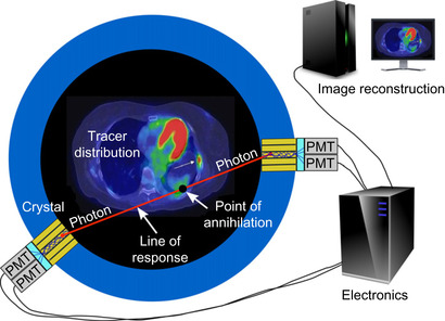 |
| Figure 42.1
A basic principle of PET imaging.
|
Although coincidence events provide line-integral measurements of the tracer distribution, histogramming these events into a sinogram is often inefficient because the number of events recorded is much smaller than the number of possible measurements, and therefore, the sinogram is sparsely filled. Instead, reconstruction is performed directly from the list-mode data, using algorithms such as
list-mode ordered-subsets expectation-maximization
(OSEM)
[9]
[10]
[11]
and
[12]
, a variation of the popular OSEM algorithm
[13]
, itself an accelerated version of the EM algorithm
[14]
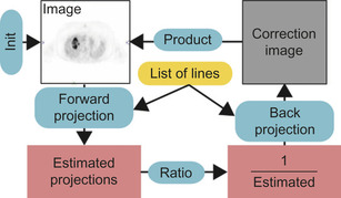
. List-mode OSEM computes the maximum likelihood estimate by iteratively applying a sequence of forward- and back-projection operations along a list of lines (Figure 42.2
).
42.1.2. Challenges
List-mode OSEM, a computationally demanding algorithm, cannot be implemented using GPU texture-mapping approaches
[2]
[3]
[4]
[5]
and
[6]
because the linear mapping between image space and projection space does not apply to a list of randomly oriented lines. Instead, lines must be processed individually, and this issue raises new, complex challenges for a GPU implementation.
One of the major obstacles is that list-mode reconstruction requires scatter operations. In principle, forward- and back-projection operations can be performed either in a
voxel-driven
or
line-driven
manner. In GPGPU language, output-driven projection operations are gather operations, whereas input-driven projection operations are scatter operations (Table 42.1
). A gather operation reads an array of data from an array of addresses, whereas a scatter operation writes an array of data to an array of addresses. For instance, a line-driven forward projection loops through all the lines and for each line, reads and sums the voxels that contribute to the line. A voxel-driven forward projection loops through all the voxels in the image and, for each voxel, updates the lines that receive contributions from the voxel. Both operations produce the same output, but data write hazards can occur in scatter operations. It has been previously suggested that, for best computing performance, the computation of line-projection operations for tomography should be output driven (i.e., gather)
[12]
.
| Forward Projection | Back Projection | |
|---|---|---|
| Line driven | Gather | Scatter |
| Voxel driven | Scatter | Gather |
In list mode, the projection lines are not ordered; therefore, only line-driven operations may be utilized. As a result, list-mode back projection requires scatter operations. In the previous version of our list-mode reconstruction code, implemented using OpenGL/Cg, the scatter operations are performed by programming in the vertex shaders where the output is written
[15]
. In that approach, a rectangular polygon is drawn into the frame-buffer object so that it encompasses the intersection of the line with the slice. This chapter presents a new approach where the output of the back projection is written directly to the slice, stored in shared memory.
Another challenge arising when performing list-mode projections on the GPU is the heterogeneous nature of the computations. As we have seen, lines stored in a list must be processed individually. However, because of the variable line length, the amount of computation per line can vary greatly. Therefore, to achieve efficient load balancing, computation must be broken down into elements smaller than the line itself.
Lastly, PET image reconstruction differs from X-ray CT because in order to reach high image quality, back projection and forward projection must model the imperfect response of the system, in particular, physical blurring processes — such as positron range and limited detector resolution. These blurring processes are implemented by projecting each line using a volumetric “tube” (Figure 42.3
) and wide, spatially varying projection kernels
[16]
and
[17]
. As a result, the number of voxels that participate in the projection of each line increases sharply, resulting in higher computational burden and increased complexity.
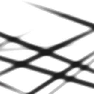 |
| Figure 42.3
An axial slice, showing the back projection of nine randomly oriented lines using a 3-D “tube” model and a radially symmetric Gaussian kernel.
|
42.2. Core Methods
To address the challenges described in the previous section, we present several novel approaches based on CUDA.
2. The image volume, which needs to be accessed randomly, is too large (>1 MB) to be stored in shared memory. Therefore, line-projection operations traverse the volume slice by slice, with slice orientation perpendicular to the predominant direction of the lines (Figure 42.4
). The three classes of lines are processed sequentially. Streaming multiprocessors (SM) load one slice at a time into shared memory, which effectively acts as a local cache (Figure 42.4
). The calculations relative to the shared slice are performed in parallel by many concurrent threads, with each thread processing one line.
3. Because lines have different lengths, more threads are assigned to longer lines. By distributing the workload both over slices and over lines, we can balance the computation load.
4. All threads execute a double for-loop over all the voxels participating in the projection (Figure 42.4
). Because lines are predominantly orthogonal to the slice, a for-loop with fixed bounds reaches all the voxels that participate in the projection while keeping the threads from diverging. More specifically, because the slice-based approach guarantees that the angle between the slice normal and the line is less than 45 degrees (Figure 42.5
), these bounds are set to
 , where
T
W
is the width of the projection tube and
S
the slice thickness, within the for-loop, the threads read (write to) all the voxels that participate for the current slice, weighting them by a kernel value computed on the fly on the GPU. The double for-loop can sometimes reach voxels that are outside the projection tube; these voxels are rejected based on their distance to the line.
, where
T
W
is the width of the projection tube and
S
the slice thickness, within the for-loop, the threads read (write to) all the voxels that participate for the current slice, weighting them by a kernel value computed on the fly on the GPU. The double for-loop can sometimes reach voxels that are outside the projection tube; these voxels are rejected based on their distance to the line.
5. Because lines can intersect, atomic add operations must be used to update voxels during back projection to avoid write data races between threads. Currently, these operations are performed in integer mode, but with the recently-released Fermi architecture, atomic operations can now be applied to floating-point values.
6. The list of lines is stored in global memory. Data transfers are optimized because the line geometry is accessed in a sequential, and therefore coalesced, manner.
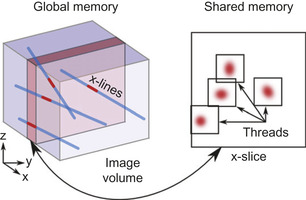 |
| Figure 42.4
Depiction of a CUDA-based line projection for a set of lines in the
x
class. The image volume and the line geometry are stored in global memory. Slices are loaded one by one into shared memory. One thread is assigned to each line to calculate the portion of the projection involved with the current slice, which involves a 2-D loop with constant bounds.
|
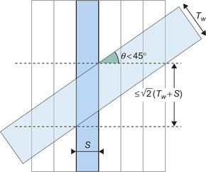 |
| Figure 42.5
Intersection of a projection tube (in gray) with a slice. Because the obliquity of the line is less than 45 degrees, the volume of intersection is bounded, and a fixed number of iterations suffice to enumerate all the voxels that participate in the projection for the current slice.
|
42.3. Implementation
42.3.1. Overview
As discussed previously, projecting a list of randomly ordered lines on the GPU raises many challenges. To our knowledge, the only implementation of list-mode reconstruction on the GPU was done by our group using OpenGL/CG
[15]
.
However, using OpenGL for GPGPU has several drawbacks: The code is difficult to develop and maintain because the algorithm must be implemented as a graphics-rendering process; performance may be compromised by OpenGL's lack of access to all the capabilities of the GPU, for example, shared memory; and code portability is limited because the code uses hardware-specific OpenGL extensions. CUDA overcomes these challenges by making the massively parallel architecture of the GPU more accessible to the developer in a C-like programming paradigm.
Briefly, the CUDA execution model organizes individual threads into thread blocks. The members of a thread block can communicate through fast shared memory, whereas threads in different blocks run independently. Atomic operations and thread synchronization functions are further provided to coordinate the execution of the threads within a block. Because the runtime environment is responsible for scheduling the blocks on the streaming multiprocessors (SMs), CUDA code is scalable and will automatically exploit the increased number of SMs on future graphics cards.
The methods described in this chapter were developed as part of our GPU line-projection library (GLPL). The GLPL is a general-purpose, flexible library that performs line-projection calculations using CUDA. It has two main features: (1) Unlike previous GPU projection implementations, it does not require lines to be organized in a sinogram and (2) A large set of voxels can participate in the projection; these voxels are located within a tube a certain distance away from the line and can be weighted by a programmable projection kernel. Collaborating with Philips Healthcare, we are currently investigating using the GLPL with their newest PET system, the Gemini TF, with so-called time-of-flight capabilities that require list-mode processing
[18]
. The GLPL is flexible and can be used for image reconstruction for other imaging modalities, such as X-ray CT and single-photon emission computed tomography (SPECT).
The GLPL implements GPU data structures for storing lines and image volumes, and primitives for performing line-projection operations. Using the GLPL, the list-mode OSEM reconstruction algorithm (Figure 42.2
) can be run entirely on the GPU. The implementation was tested on an NVIDIA GeForce 285 GTX with compute capability 1.3.
42.3.2. Data Structures
Image volumes are stored in global memory as 3-D arrays of 32-bit floats. For typical volume sizes, the image does not fit in the fast shared memory. For instance, the current reconstruction code for the Gemini TF uses matrices with 72 × 72 × 20 coefficients for storing the images, thus occupying 405 kB in global memory. However, individual slices can be stored in shared memory, which acts as a managed cache for the global memory (Figure 42.4
).
By slicing the image volume in the dimension most orthogonal to the line orientation, the number of voxels included in the intersection of the projection tube with the current slice is kept bounded (Figure 42.5
). To exploit this property, the lines are divided into three classes, according to their predominant orientation which is determined by calculating an inner product. Each of the three classes is processed sequentially by different CUDA kernels. Because PET detectors are typically arranged in a cylindrical geometry, with axial height short compared with diameter, the
z
class is empty and only slices parallel to the
x
−
z
or
y
−
z
planes are considered. For the image volume specifications used in this work, these slices are 5.6 kB and easily fit in 16 kB of shared memory.
The list of lines is stored in the GPU global memory, where each line is represented as a pair of indices using two 16-bit unsigned integers. A conversion function maps the indices to physical detector coordinates. The Philips Gemini TF PET system has, for instance, 28,336 individual detectors, organized in 28 modules, with each module consisting of a 23 × 44 array of 4 × 4 × 22 mm
3
crystals
[15]
. A 5 minutes. PET dataset can contain hundreds of millions of lines and occupy hundreds of megabytes in global memory.
Lines are processed sequentially and, therefore, the geometry data are coherently accessed by the threads. To perform a projection, each thread first reads the two detector indices that define the line end points from global memory. The memory access is coalesced; hence, on a device of compute capability 1.3, two 128-bit memory transactions are sufficient for a half-warp (i.e., eight threads running concurrently on the same SM). The indices are then converted into geometrical coordinates by arithmetic calculations.
42.3.3. Forward Projection
The line-forward projection, mathematically a sparse matrix-vector multiplication, is a gather operation. The voxel values contained in a tube centered on the line are read, weighed by a projection kernel, and accumulated. A basic CPU implementation would employ three levels of nested loops with variable bounds.
However, such an approach is not efficient in CUDA because the computational load would be unevenly distributed. Instead, the outer level of the nested loops is performed in parallel by assigning one thread per line and per slice. Because the lines have been partitioned according to their orientation, the angle between the slice normal and the line is less than 45degrees (Figure 42.5
), and all the voxels in the tube (of width
T
W
) can be reached when the number of iterations in each of the two inner for-loops is set to
 . Hence, the computation load is homogeneously distributed onto the many cores. Having all the threads run the same number of iterations is a critical feature of our implementation. If threads ran a different number of iterations, their execution would diverge. Furthermore, having constant bounds allows the 2-D for-loop to be unrolled, providing additional acceleration.
Source code for the forward-projection kernel is given in
Figure 42.6
. First, the threads collaboratively load the image slice into shared memory. After each thread reads out the coordinates of the line, the 2-D for-loop is performed. Within the loop, voxel values are read from shared memory. These values are weighted by a projection kernel, computed locally, and accumulated within a local register. In our implementation, we used a Gaussian function, parameterized by the distance between the voxel center and the line, as a projection kernel. The Gaussian kernel is computed using fast GPU-intrinsic functions. The final cumulative value is accumulated in global memory.
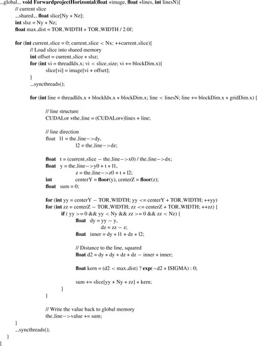 |
| Figure 42.6
A CUDA kernel used to perform forward projection of horizontal lines.
|
42.3.4. Back Projection
Back projection, mathematically the transpose operation of forward projection, smears the lines uniformly across the volume image (Figure 42.3
). Back projection is therefore, in computation terms, a scatter operation. Such scatter operations can be implemented explicitly in the CUDA programming model because write operations can be performed at arbitrary locations.
The CUDA implementation of line back projection is modeled after the forward projection. There are, however, two basic differences. First, the current slice is cleared beforehand and written back to the global memory thereafter. Second, the threads update voxels in the slice instead of reading voxel data. Because multiple threads might attempt to update simultaneously the same voxel, atomic add operations are used.
42.4. Evaluation and Validation of Results, Total Benefits, and Limitations
42.4.1. Processing Time
The GLPL was benchmarked for speed and accuracy against a CPU-based reference implementation. The processing time was measured for the back projection and forward projection of one million spatially random lines, using an image volume of size 72 × 72 ×20 voxels and included the transfer of line and image data from the CPU to the GPU. The CPU implementation was based on the ray-tracing function currently employed in the Gemini TF reconstruction software. The hardware used in this comparison was a GeForce 285GTX for the GPU and an Intel Core2 E6600 for the CPU. The GPU and CPU implementations processed one million lines in 0.46s and 20s, respectively. The number of thread blocks was varied and the total processing time split into GPU-CPU communication, GPU processing, and CPU processing (Figure 42.7
).
 |
| Figure 42.7
Runtime for processing 1 million lines with CUDA as a function of the number of thread blocks.
|
In the current implementation of the GLPL, most of the processing time is spent on GPU computation (Figure 42.7
). Furthermore, data is transferred only once from the CPU to the GPU and used multiple times by the GPU over multiple iterations. Likewise, some of the preprocessing tasks are performed by the CPU only once for the entire reconstruction.
As expected, only the GPU computation time depends upon the number of thread blocks. The total throughput (expressed in number of lines processed per second) improves with increasing number of blocks, until reaching a plateau at 30 blocks (Figure 42.8
). This result is expected because the GeForce 285 GTX can distribute thread blocks onto 30 SMs. When fewer than 30 blocks are scheduled, the overall compute performance is decreased because some of the SMs are idle. At the peak, the GLPL is able to process 2 million lines per second.
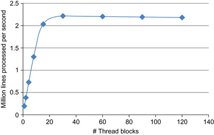 |
| Figure 42.8
Performance of the GPU implementation, measured in million lines per second, as a function of the number of thread blocks.
|
In order to gain more insight, we modeled the processing time
T
proc
as the sum of three components:
 where
S
is the scalable computation load,
N
the number of SM used,
C
the constant overhead (including CPU processing and CPU-GPU communication), and
k
the computation overhead per SM used. We found that for one million lines, the scalable computation load was
S
= 5027 ms, the constant overhead
C
= 87 ms, and the overhead per SM
k
= 6 ms. The goodness of the fit was
r
2
= 0.9998. Hence, 95% of all computation is scalable and runs in parallel.
where
S
is the scalable computation load,
N
the number of SM used,
C
the constant overhead (including CPU processing and CPU-GPU communication), and
k
the computation overhead per SM used. We found that for one million lines, the scalable computation load was
S
= 5027 ms, the constant overhead
C
= 87 ms, and the overhead per SM
k
= 6 ms. The goodness of the fit was
r
2
= 0.9998. Hence, 95% of all computation is scalable and runs in parallel.
42.4.2. Line-Projection Accuracy
The accuracy of the GLPL was compared with a standard CPU implementation of line-projection operations by running list-mode OSEM on both platforms. Because the development of data conversion tools for the Philips Gemini TF is still under way, we measured the accuracy of the line projections on a dataset acquired with another system installed at Stanford, the GE eXplore Vista DR, a high-resolution PET scanner for small animal preclinical research.
A cylindrical “hot rod” phantom, comprising rods of different diameters (1.2, 1.6, 2.4, 3.2, 4.0, and 4.8 mm) was filled with 110 μCi of a radioactive solution of Na
18
F and 28.8 million lines were acquired. Volumetric images, of size 103 × 103 × 36 voxels, were reconstructed using the list-mode 3-D OSEM algorithm. For simplicity, the usual data corrections (for photon scatter, random coincidences, photon attenuation, and detector efficiency normalization) were not applied. For this image configuration, each subiteration (forward projection, back projection, and multiplicative update) took 746ms per million LORs, including 489ms for calculation on the GPU, 210 ms for preprocessing on the CPU, and 46ms for communication between the CPU and the GPU. The entire reconstruction took 1.3 minutes on the GPU and about 4.3 hours on the CPU. Note that for the accuracy validation, the reference CPU reconstruction was performed with nonoptimized research code because the fast ray-tracing functions used in the Gemini TF system (and used for measuring processing time) could not be easily ported to the eXplore Vista system.
Transaxial image slices, reconstructed using the CPU and the GPU, are visually identical (Figure 42.9
). The RMS deviation between both images is 0.08% after five iterations, which is negligible compared with the statistical variance of the voxel values in a typical PET scan (> 10%, from Poisson statistics). Higher image quality can be achieved by decreasing the number of subsets and increasing the number of iterations (Figure 42.9c
). Such reconstruction is only practical on the GPU because of the increased computational cost.
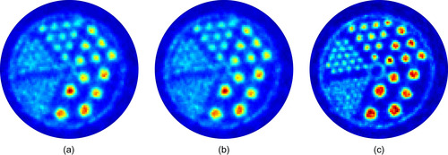 |
| Figure 42.9
Hot rods phantom, acquired on a preclinical PET scanner with two iterations and 40 subsets of list-mode OSEM, using CPU-based projections (a) and the GLPL (b). A better image can be obtained using five subsets and 20 iterations on the GPU (c).
|
We believe that the small deviation that we measured was caused by small variations in how the arithmetic operations are performed on the CPU and GPU. For example, we have observed that the exponential function produces slightly different results on each platform. These differences are amplified by the ill-posed nature of the inverse problem solved by the iterative image reconstruction algorithm.
As an example of a real application, a mouse was injected with Na
18
F, a PET tracer, and imaged on the eXplore Vista (Figure 42.10
). Image reconstruction was performed with 16 iterations and five subsets of list-mode OSEM using the GLPL.
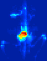 |
| Figure 42.10
Mouse PET scan (maximum intensity projection), reconstructed with 16 iterations and five subsets of list-mode OSEM using the GLPL.
|
42.5. Future Directions
A current limitation of our implementation is the size of the GPU shared memory. In particular, in high-resolution PET, images are stored with finer sampling, and slices might not be fit in shared memory (16 kB). As the amount of shared memory increases with the release of new GPUs, the GLPL will be able to process larger images and/or process multiple contiguous image slices simultaneously. With the recent release of the Fermi architecture, which offers 48 kB of shared memory, slices taken from image volumes as large as 175 × 175 × 60 voxels can be loaded into shared memory. Alternatively, the image volume can be processed directly in global memory, or the image slices can be subdivided into smaller blocks that fit within shared memory. Both approaches, however, would diminish compute efficiency.
The number of line events generated in a typical PET scan — approximately 20 million per minute — raises tremendous challenges for distributing, storing, and processing such a large amount of data. Hence, we are designing a parallel architecture that distributes the stream of line events onto a cluster of GPU nodes for reconstruction.
References
[1]
G.T. Herman,
Fundamentals of Computerized Tomography: Image Reconstruction from Projections
.
second ed.
(2009
)
Springer
,
London, UK
.
[2]
B. Cabral, N. Cam, J. Foran,
Accelerated volume rendering and tomographic reconstruction using texture mapping hardware
,
In: (Editors: A. Kaufman, W. Krueger)
Proceedings of the 1994 Symposium on Volume Visualization, 17–18 October 1994
Washington, DC
. (1994
)
ACM
,
New York
.
[3]
F. Xu, K. Mueller,
Accelerating popular tomographic reconstruction algorithms on commodity PC graphics hardware
,
IEEE Trans. Nucl. Sci.
52
(2005
)
654
.
[4]
J. Kole, F. Beekman,
Evaluation of accelerated iterative X-ray CT image reconstruction using floating point graphics hardware
,
Phys. Med. Biol.
51
(2006
)
875
.
[5]
F. Xu, K. Mueller,
Real-time 3D computed tomographic reconstruction using commodity graphics hardware
,
Phys. Med. Biol.
52
(2007
)
3405
.
[6]
P. Despres, M. Sun, B.H. Hasegawa, S. Prevrhal,
FFT and cone-beam CT reconstruction on graphics hardware
,
In: (Editors: J. Hsieh, M.J. Flynn)
Proceedings of the SPIE, 16 March 2007
San Diego, CA, SPIE, Bellingham, WA
. (2007
), p.
6510
.
[7]
J.M. Ollinger, J.A. Fessler,
Positron-emission tomography
,
IEEE Signal Process
14
(1
) (1997
)
43
.
[8]
S. Gambhir,
Molecular imaging of cancer with positron emission tomography
,
Nat. Rev. Cancer
2
(2002
)
683
–
693
.
[9]
L. Parra, H.H. Barrett,
List-mode likelihood: EM algorithm and image quality estimation demonstrated on 2-D PET
,
IEEE Trans. Med. Image
17
(1998
)
228
.
[10]
A.J. Reader, S. Ally, F. Bakatselos, R. Manavaki, R.J. Walledge, A.P. Jeavons, P.J. Julyan, S. Zhao, D.L. Hastings, J. Zweit,
One-pass list-mode EM algorithm for high-resolution 3-D PET image reconstruction into large arrays
,
IEEE Trans. Nucl. Sci.
49
(2002
)
693
.
[11]
R.H. Huesman,
List-mode maximum-likelihood reconstruction applied to positron emission mammography (PEM) with irregular sampling
,
IEEE Trans. Med. Image
19
(2000
)
532
.
[12]
A. Rahmim, J.C. Cheng, S. Blinder, M.L. Camborde, V. Sossi,
Statistical dynamic image reconstruction in state-of-the-art high-resolution PET
,
Phys. Med. Biol.
50
(2005
)
4887
.
[13]
H. Hudson, R. Larkin,
Accelerated image reconstruction using ordered subsets of projection data
,
IEEE Trans. Med. Image
13
(1994
)
601
.
[14]
L.A. Shepp, Y. Vardi,
Maximum-likelihood reconstruction for emission tomography
,
IEEE Trans. Med. Image
2
(1982
)
113
.
[15]
G. Pratx, G. Chinn, P.D. Olcott, C.S. Levin,
Fast, accurate and shift-varying line projections for iterative reconstruction using the GPU
,
IEEE Trans. Med. Image
28
(3
) (2009
)
435
.
[16]
A. Alessio, P. Kinahan, T. Lewellen,
Modeling and incorporation of system response functions in 3-D whole body PET
,
IEEE Trans. Med. Image
25
(2006
)
828
.
[17]
V.Y. Panin, F. Kehren, C. Michel, M.E. Casey,
Fully 3D PET reconstruction with system matrix derived from point source measurements
,
IEEE Trans. Med. Image
25
(7
) (2006
)
907
.
[18]
S. Surti, S. Karp, L. Popescu, E. Daube-Witherspoon, M. Werner,
Investigation of time-of-flight benefits for fully 3-D PET
,
IEEE Trans. Med. Image
25
(2006
)
529
.
..................Content has been hidden....................
You can't read the all page of ebook, please click here login for view all page.