
Paulius MicikeviciusArmstrong Atlantic State University
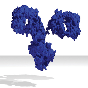
Determining protein 3D structure is one of the greatest challenges in computational biology. Nuclear magnetic resonance (NMR) spectroscopy is the second most popular method (after X-ray crystallography) for structure prediction. Given a molecule, NMR experiments provide upper and lower bounds on the interatomic distances. If all distances are known exactly, Cartesian coordinates for each atom can be easily computed. However, only a fraction (often fewer than 10 percent) of all distance bounds are obtained by NMR experiments (unknown upper and lower bounds are set to the molecule’s diameter and the diameter of a hydrogen atom, respectively). Thus, a number of heuristics are used in practice to generate 3D structures from NMR data. Because the quality of the computed structures and the time required to obtain them depend on the bound tightness, it is necessary to use efficient procedures for bound smoothing (that is, increasing lower bounds or decreasing upper bounds). The most widely used procedure is based on the triangle inequality and is included in popular molecular dynamics software packages, such as X-PLOR and DYANA. In this chapter we describe a GPU implementation of the triangle inequality distance-bound smoothing procedure. Figure 43-1 shows one example of results obtained.
An n-atom molecule is modeled with a complete graph on n nodes, Kn, where nodes represent atoms. Each edge (i, j) is assigned two labels—upper and lower bounds, denoted by uij and lij, on the distance between the ith and jth atoms. Let i, j, and k be arbitrary points in three-dimensional Euclidean space. The distances between points, dij, dik, and dkj must satisfy the triangle inequality; for example, dij ≤ dik + dkj. The triangle inequality can also be stated in terms of the upper and lower bounds on the distances. The upper bound on dij must satisfy the inequality uij ≤ uik + ukj, while the lower bound must satisfy lij ≥ max {lik- ukj, lkj- uik}. Upper bounds must be tightened first, because lower values for upper bounds will lead to larger lower bounds. Dress and Havel (1988) have shown that violation of the triangle inequality can be eliminated in O(n3) time by means of a Floyd-Warshall-type algorithm for the all-pairs shortest-paths problem.
Given a weighted graph on n nodes, the all-pairs shortest-paths problem asks to find the shortest distances between each pair of nodes. The problem is fundamental to computer science and graph theory. In addition to bound smoothing, it has other practical applications, such as network analysis and solving a system of difference constraints (Cormen et al. 2001). A number of sequential approaches exist for solving the all-pairs shortest-paths problem (for a brief discussion, see Bertsekas 1993), but the Floyd-Warshall algorithm is generally favored for dense graphs due to its simplicity and an efficient memory-access pattern. The sequential Floyd-Warshall algorithm is shown in Algorithm 43-1 (we assume that the nodes are labeled with integers 1, 2, . . ., n). We assume that a graph is stored as a 2D distance matrix D, where D[i, j] contains the distance between nodes i and j. The Floyd-Warshall algorithm requires O(n3) time and O(n2) storage. The upper-bound smoothing algorithm is obtained by replacing line 4 of Algorithm 43-1 with uij ← min {uij, uik + ukj}. Similarly, the algorithm for tightening lower bounds is obtained by replacing line 4 with lij ← max {lij, lik − ukj, lkj − uik}.
A classic parallelization for O(n2) processors is shown in Algorithm 43-2, where Pij refers to the processor responsible for updating the distance dij.
The parallelization in Algorithm 43-2 is amenable to a GPU implementation because each processor reads from multiple locations but writes to one predetermined location.
To be solved on the GPU, the distance-bound smoothing problem is formulated as a rendering task for the programmable fragment unit. Both the lower and the upper bounds are stored as separate 2D textures. Although such a storage choice wastes memory (texels (i, j) and (j, i) contain the same value), it leads to fewer texture fetches in vectorized implementations, and thus to higher performance, as described later in Section 43.3.4. For simplicity of presentation, we first describe the scalar version of the algorithm, leaving the vectorization for the end of the section.
Because of the dynamic nature of the Floyd-Warshall algorithm, the output of iteration k is the input for iteration (k + 1). Although this requires no special considerations when programming for a CPU, current GPU architectures do not allow the same memory block to be a render target and a texture at the same time. We overcome this constraint with ping-pong buffering: rendering alternates between the front and back buffers. For example, we render to the front buffer when the back buffer is bound as a texture. The functions of the buffers are flipped in the next iteration, and the process is repeated. Because there is no memory copy, we have experimentally confirmed that ping-pong buffering is twice as fast as a copy-to-texture approach.
An all-pairs shortest-paths solution for a graph with n nodes is computed by rendering an n×n pixel square in n passes, each corresponding to a single iteration of the for loop on line 1 in Algorithm 43-2. The pixel in position (i, j) corresponds to distance dij. Thus, a fragment shader performs the computation corresponding to line 3 in Algorithm 43-2. In the naive implementation, given distance dij, the shader generates two sets of texture coordinates to index the storage for distances dik and dkj, and then performs algebraic operations. Performance is improved by moving the texture coordinate generation from the shader to the rasterizer: during the kth iteration, the four vertices of the rectangle are each assigned three texture coordinates, as shown in Figure 43-2a. Thus, after interpolation, every fragment (i, j) receives the necessary three texture coordinates. Moving texture coordinate generation from the shader to the rasterizer increased the performance by approximately 10 percent.
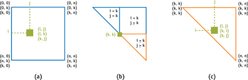
The upper and lower distance bounds can be stored respectively in the upper and lower triangles of a texture. Under this assumption, it is necessary to ensure that the shader for smoothing the upper bounds fetches only the upper-triangle texels. This is achieved when texture coordinate (u, v) satisfies u < v: during the kth iteration, the upper triangle is partitioned into three regions determined by the relation between i, j, and k, as shown in Figure 43-2b. Thus, three geometric primitives are rendered with texture coordinates adjusted according to the region. For example, texture coordinates for the bottom triangle are shown in Figure 43-2c. If a single primitive is rendered instead of three as described, the GPU has to execute additional instructions for each fragment to determine to which region the fragment belongs. A similar approach can be used to smooth the lower bounds.
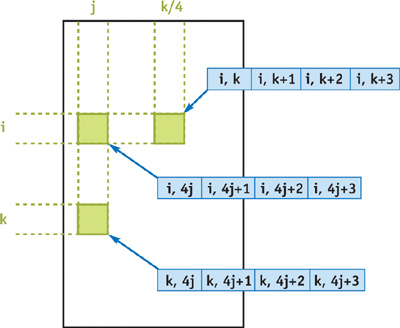
We can improve performance by vectorizing the algorithm, because each of the GPU pipelines operates on four-component vectors. We can do so by packing the distances of four consecutive edges into RGBA components of a single texel. As shown in Figure 43-3, texel T[i, j] contains the following entries of the distance matrix: D[i, 4j], D[i, 4j + 1], D[i, 4j + 2], D[i, 4j + 3]. Thus, only an n×n/4 rectangle needs to be rendered. Note that rendering pixels in the ith row during the kth iteration requires fetching the distance value D[i, k], so we need to modify the computation for the upper-bound smoothing,
D[i, j] ← min{D[i, j], D[i, k] + D[k, j]}, |
for vector operations:
T[i, j] ← min{T[i, j],Ψ+T[k, j]}, |
where ψ is a vector created by replicating the R, G, B, or A component value of T[i, [k/4]], depending on whether k ≡ 0, 1, 2, or 3 (mod 4), respectively. The code for smoothing the lower bounds is modified similarly. Generating the ψ vector on the GPU can be expensive because under certain circumstances, branching or integer operations are inefficient in current fragment units. We can overcome this limitation by running four separate shader programs, each hard-coded for a different value of k mod 4, thus avoiding branching and integer operations (replicating a scalar value across the ψ does not impose any additional cost [Mark et al. 2003]). The OpenGL application must explicitly bind the appropriate shader program for each of the n iterations, with a negligible overhead.
Although the upper and lower distance bounds could be stored in the upper and lower triangles, respectively, of the same 2D texture, this would lead to more texture fetches. For example, to update the upper bounds in texel T[i, j], we need to ensure that fetching T[k, j] returns the upper bounds on distances D[k, 4j], D[k, 4j + 1], D[k, 4j + 2], and D[k, 4j + 3]. However, if k > j, the texel T[k, j] is in the lower triangle and contains the lower bounds. As a result, we would need to fetch 4 texels (T[4j, k], T[4j+ 1, k], T[4j + 2, k], T[4j + 3, k]) instead of 1. This approach would require 11 texture fetches for each lower bound and either 3 (when i, j < k) or 6 (when i, j, or both are greater than k) texture fetches for each upper bound. Thus, we achieve better performance by storing 2 textures and rendering twice as many fragments as theoretically necessary, because 3 and 5 texture fetches are required when smoothing the upper and lower bounds, respectively.
We conducted the experiments on a 2.4 GHz Intel Xeon-based PC with 512 MB RAM and an NVIDIA GeForce 6800 Ultra GPU. The GeForce 6800 Ultra has 16 fragment pipelines, each operating on four-element vectors at 425 MHz. The applications were written in ANSI C++ using OpenGL, GLUT, and Cg (Mark et al. 2003) for graphics operations. The pbuffers, textures, and shader programs all used 32-bit IEEE-standard floating-point types, because precision is critical to distance-bound smoothing. The executables were compiled using the Intel C++ 8.1 compiler with SSE2 optimizations enabled. Furthermore, the CPU implementation was hand-optimized to minimize cache misses.
The timing results for problem sizes 128 to 4096 are shown in Table 43-1. We show the overall times as well as separate times for smoothing the lower and upper bounds. The maximum size was dictated by the graphics system, because no pbuffer larger than 4096×4096 could be allocated. All results are in milliseconds and were computed by averaging 1000 (for n = 128, 256), 100 (for n = 512), 10 (for n = 1024, 2048), or 1 (for n = 4096) consecutive executions. The compiled shaders for smoothing the lower and upper bounds consisted of nine and five assembly instructions, respectively.
Table 43-1. Times for the Optimized GPU Implementation
Time (ms) | Speedup | ||||||||
|---|---|---|---|---|---|---|---|---|---|
CPU | GPU | GPU | |||||||
Size | Lower | Upper | Overall | Lower | Upper | Overall | Lower | Upper | Overall |
128 | 4.8 | 5.5 | 10.3 | 2.1 | 2.0 | 4.1 | 2.3 | 2.7 | 2.5 |
256 | 36.4 | 40.0 | 76.4 | 9.7 | 5.4 | 15.1 | 3.8 | 7.4 | 5.1 |
512 | 517.2 | 393.3 | 910.5 | 69.7 | 35.3 | 105.0 | 7.4 | 11.1 | 8.7 |
1024 | 3,828.0 | 2,937.5 | 6,765.5 | 531.7 | 266.6 | 798.3 | 7.2 | 11.0 | 8.5 |
2048 | 29,687.0 | 22,560.9 | 52,247.9 | 4,156.2 | 2,084.3 | 6,240.5 | 7.1 | 10.8 | 8.4 |
4096 | 233,969.0 | 183,281.0 | 417,250.0 | 32,969.0 | 16,610.0 | 49,579.0 | 7.1 | 11.0 | 8.4 |
The GPU implementation of the distance-bound smoothing procedure achieves a speedup of more than eight when compared to a CPU-only implementation. This is due to the parallel nature as well as high memory bandwidth of graphics hardware. Further work can proceed in two directions: (1) designing algorithms to accommodate GPU memory limitations in order to increase the solvable problem size (4096 atoms is a modest size for a protein molecule) and (2) overlapping the computation between the CPU and the GPU.
To overcome the 4096×4096 pbuffer size restriction, the algorithm should be designed so that segments (stripes or blocks) of the adjacency matrix can be updated one at a time. Thus, the adjacency matrix would be distributed among several pixel buffers. An application-specific method for explicitly caching data in the GPU memory should also be developed to overcome the physical restriction on GPU memory. Alternatively, a recursive approach similar to the one in Park et al. 2002 could be adopted, with the GPU executing the base cases.
Sharing the computation load between the CPU and the GPU will require data transfer between the GPU and CPU memories n times for a graph on n nodes. However, the overhead may be acceptable because for each of n iterations, only one row and one column need to be communicated. Thus, communication cost is O (n2) while computation complexity is O(n3).
The author would like to thank Mark Harris and Rayann Kovacik for helpful suggestions.