A CUDA-Based Test Suit
12.1 Overview
Proposed algorithms are usually tested on benchmark for comparing both performance and efficiency. However, as it can be a very tedious task to select and implement test functions rigorously. Thanks to graphics processing units’ (GPUs) massive parallelism, a GPU-based optimization function suit will be beneficial to test and compare various optimization algorithms.
Based on the well-known CPU-based benchmarks presented in [58, 110, 109], a compute unified device architecture (CUDA)-based real parameter optimization benchmark, called cuROB, was proposed in [48]. Thanks to the great computing power of GPUs, cuROB has been of great help for optimization related tasks [47].
In the current release of cuROB, a set of single-objective real-parameter optimization functions are defined and implemented. It is a great start, as research on the single-objective optimization algorithms is the basis of the research on more complex optimization algorithms such as constrained optimization algorithms, multiobjective optimizations algorithms, and so forth.
In cuROB, the test functions are selected according to the following criteria: (1) the functions should be scalable in dimension so that algorithms can be tested under various complexities; (2) the expressions of the functions should be with good parallelism, thus efficient implementation is possible on GPUs; (3) the functions should be comprehensible such that algorithm behaviors can be analyzed in the topological context; (4) last but most important, the test suit should cover functions of various properties in order to get a systematic evaluation of the optimization algorithms.
The source code and a sample can be freely download from https://github.com/DingKe/cuROB.
12.1.1 Symbol Conventions and Definitions
Symbols and definitions used in this book are described as follows. By default, all vectors refer to column vectors which are depicted by lowercase letter and typeset in bold.
• [·] indicates the nearest integer value
• ⌊·⌋ indicates the largest integer less than or equal to
• xi denotes ith element of vector x
• f(·), g(·) and G(·) denote multivariable functions
• fopt denotes optimal (minimal) value of function f
• xopt denotes optimal solution vector, such that f(xopt) = fopt
• R denotes normalized orthogonal matrix for rotation
• D denotes dimension
• 1 = (1,…, 1)T denotes all one vector
12.1.2 General Setup
The general setup of the test suit is presented as follows:
• Dimensions: The test suit is scalable in terms of dimension. Within the hardware limit, any dimension D ≥ 2 works. However, to construct a real hybrid function, D should be at least 10.
• Search Space: All functions are defined and can be evaluated over ![]() , while the actual search domain is given as [−100, 100]D.
, while the actual search domain is given as [−100, 100]D.
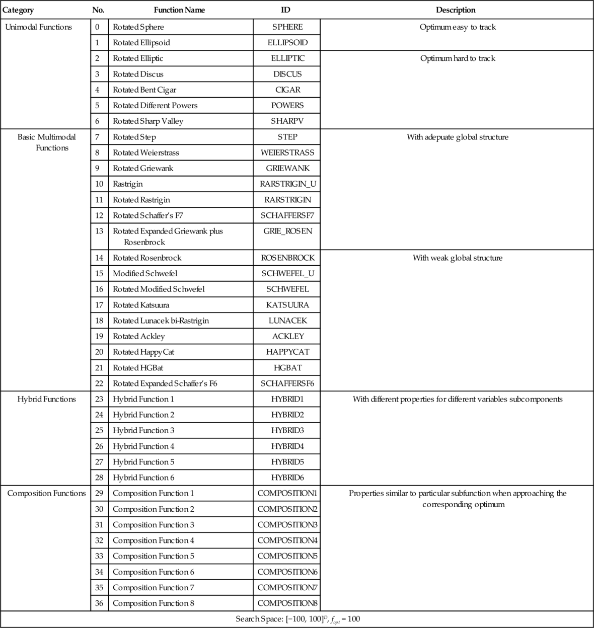
• fopt: All functions, by definition, have a minimal value of 0, a bias (fopt) can be added to each function. The selection can be arbitrary, fopt for each function in the test suit is listed in Table 12.1.
Table 12.1
Summary of cuROB’s Test Functions
| Category | No. | Function Name | ID | Description |
| Unimodal Functions | 0 | Rotated Sphere | SPHERE | Optimum easy to track |
| 1 | Rotated Ellipsoid | ELLIPSOID | ||
| 2 | Rotated Elliptic | ELLIPTIC | Optimum hard to track | |
| 3 | Rotated Discus | DISCUS | ||
| 4 | Rotated Bent Cigar | CIGAR | ||
| 5 | Rotated Different Powers | POWERS | ||
| 6 | Rotated Sharp Valley | SHARPV | ||
| Basic Multimodal Functions | 7 | Rotated Step | STEP | With adepuate global structure |
| 8 | Rotated Weierstrass | WEIERSTRASS | ||
| 9 | Rotated Griewank | GRIEWANK | ||
| 10 | Rastrigin | RARSTRIGIN_U | ||
| 11 | Rotated Rastrigin | RARSTRIGIN | ||
| 12 | Rotated Schaffer’s F7 | SCHAFFERSF7 | ||
| 13 | Rotated Expanded Griewank plus Rosenbrock | GRIE_ROSEN | ||
| 14 | Rotated Rosenbrock | ROSENBROCK | With weak global structure | |
| 15 | Modified Schwefel | SCHWEFEL_U | ||
| 16 | Rotated Modified Schwefel | SCHWEFEL | ||
| 17 | Rotated Katsuura | KATSUURA | ||
| 18 | Rotated Lunacek bi-Rastrigin | LUNACEK | ||
| 19 | Rotated Ackley | ACKLEY | ||
| 20 | Rotated HappyCat | HAPPYCAT | ||
| 21 | Rotated HGBat | HGBAT | ||
| 22 | Rotated Expanded Schaffer’s F6 | SCHAFFERSF6 | ||
| Hybrid Functions | 23 | Hybrid Function 1 | HYBRID1 | With different properties for different variables subcomponents |
| 24 | Hybrid Function 2 | HYBRID2 | ||
| 25 | Hybrid Function 3 | HYBRID3 | ||
| 26 | Hybrid Function 4 | HYBRID4 | ||
| 27 | Hybrid Function 5 | HYBRID5 | ||
| 28 | Hybrid Function 6 | HYBRID6 | ||
| Composition Functions | 29 | Composition Function 1 | COMPOSITION1 | Properties similar to particular subfunction when approaching the corresponding optimum |
| 30 | Composition Function 2 | COMPOSITION2 | ||
| 31 | Composition Function 3 | COMPOSITION3 | ||
| 32 | Composition Function 4 | COMPOSITION4 | ||
| 33 | Composition Function 5 | COMPOSITION5 | ||
| 34 | Composition Function 6 | COMPOSITION6 | ||
| 35 | Composition Function 7 | COMPOSITION7 | ||
| 36 | Composition Function 8 | COMPOSITION8 | ||
| Search Space: [−100, 100]D, fopt = 100 | ||||
• xopt: The optimum point of each function is located at original, which is randomly distributed in [−70, 70]D, and is selected as the new optimum.
• Rotation Matrix: To derive nonseparable functions from separable ones, the search space is rotated by a normalized orthogonal matrix R. For a given function in one dimension, a different R is used. Variables are divided into three (almost) equal-sized subcomponents randomly. The rotation matrix for each subcomponent is generated from standard normally distributed entries by Gram–Schmidt orthonormalization. Then, these matrices consist of the R actually used.
12.1.3 CUDA Interface and Implementation
A simple description of the interface and implementation is given below. For detail, see the source code and its accompanied readme file.
12.1.3.1 Interface
Only benchmark.h needs to be included to access the test functions, and the CUDA file benchmark.cu needs be compiled and linked. Before the compiling start, two macro, DIM and MAX_CONCURRENCY should be modified accordingly. DIM defines the dimension of the test suit to be used while MAX_CONCURRENCY defines the number of function evaluations which can be invoked concurrently. As memory needed to be pre-allocated, MAX_CONCURRENCY should not exceed the hardware limit.
Host interface function initialize () accomplish all initialization tasks, so must be called before any test function can be evaluated. Allocated resource is released by host interface function dispose ().
Both double precision (DP) and single precision (SP) are supported through func_evaluate () and func_evaluatef () respectively. Take note that device pointers should be passed to these two functions. For the convenience of CPU code, C interfaces are provided, with h_func_evaluate () for DP and h_func_evaluatef () for SP. (In fact, they are just wrappers of the GPU interfaces.)
12.1.3.2 Efficiency Considerations
When configuration of the suit, some should be taken care for the sake of efficiency. It is better to evaluate a batch of vectors. Dimensions of fold of 32 (the warp size) can more efficient. For example, dimension of 96 is much more efficient than 100, even though 100 is just little greater than 96.
12.1.4 Test Suite Summary
The whole of the test functions fall into four categories: unimodal functions, basic multimodal functions, hybrid functions, and composition functions. The summary of the suit is listed in Table 12.1. Detailed information of each function will be given in the following sections.
12.2 Speedup and Baseline Results
With different hardware, various speedups can be achieved. Thirty functions are the same as CEC’14 benchmark. We test the cuROB’s speedup with these 30 functions under the following settings: Windows 7 SP1 x64 running on Intel i5-2310 CPU with NVIDIA 560 Ti, the CUDA version is 5.5. Fifty evaluations were performed concurrently and repeated 1000 runs. The evaluation data were generated randomly from uniform distribution.
The speedups with respect to different dimensions are listed in Tables 12.2 (SP) and 12.3 (DP). Notice that the corresponding dimensions of cuROB are 10, 32, 64, and 96, respectively, and the numbers are the same in Table 12.1.
Table 12.2
Speedup (Single Precision) With Different Dimensions
| D | No. 3 | No. 4 | No. 5 | No. 8 | No. 9 | No. 10 | No. 11 | No. 13 | No. 14 | No. 15 |
| 10 | 0.59 | 0.20 | 0.18 | 12.23 | 0.49 | 0.28 | 0.31 | 0.32 | 0.14 | 0.77 |
| 32 | 3.82 | 2.42 | 2.00 | 47.19 | 3.54 | 1.67 | 3.83 | 5.09 | 2.06 | 3.54 |
| 64 | 4.67 | 2.72 | 2.29 | 50.17 | 3.56 | 0.93 | 3.06 | 2.88 | 2.20 | 3.39 |
| 94 | 13.40 | 10.10 | 8.50 | 84.31 | 11.13 | 1.82 | 9.98 | 9.66 | 8.75 | 6.73 |
| D | No. 16 | No. 17 | No. 19 | No. 20 | No. 21 | No. 22 | No. 23 | No. 24 | No. 25 | No. 26 |
| 10 | 0.80 | 3.25 | 0.36 | 0.20 | 0.26 | 0.45 | 0.63 | 0.44 | 2.80 | 0.52 |
| 32 | 5.57 | 10.04 | 3.46 | 1.22 | 1.42 | 6.44 | 3.95 | 3.43 | 11.47 | 3.36 |
| 64 | 5.45 | 13.19 | 3.27 | 2.10 | 2.27 | 3.81 | 4.62 | 3.07 | 14.17 | 3.34 |
| 96 | 14.38 | 23.68 | 11.32 | 8.26 | 8.49 | 11.60 | 13.67 | 10.64 | 30.11 | 10.71 |
| D | No. 27 | No. 28 | No. 29 | No. 30 | No. 31 | No. 32 | No. 33 | No. 34 | No. 35 | No. 36 |
| 10 | 0.65 | 0.72 | 0.70 | 0.55 | 0.71 | 3.49 | 3.50 | 0.84 | 1.28 | 0.70 |
| 32 | 2.73 | 3.09 | 3.63 | 3.10 | 4.10 | 12.39 | 12.51 | 5.25 | 5.19 | 3.33 |
| 64 | 3.86 | 4.01 | 3.21 | 2.67 | 3.38 | 12.68 | 12.63 | 3.80 | 5.27 | 3.13 |
| 96 | 12.04 | 11.32 | 8.15 | 6.27 | 8.49 | 23.67 | 23.64 | 9.50 | 11.79 | 7.93 |

Table 12.3
Speedup (Double Precision) With Different Dimensions
| D | No. 3 | No. 4 | No. 5 | No. 8 | No. 9 | No. 10 | No. 11 | No. 13 | No. 14 | No. 15 |
| 10 | 0.56 | 0.19 | 0.17 | 9.04 | 0.43 | 0.26 | 0.29 | 0.30 | 0.14 | 0.75 |
| 32 | 3.78 | 2.43 | 1.80 | 33.37 | 3.09 | 1.59 | 3.52 | 4.81 | 1.97 | 3.53 |
| 64 | 4.34 | 2.49 | 1.93 | 30.82 | 3.15 | 0.92 | 2.87 | 2.74 | 2.11 | 3.29 |
| 96 | 12.27 | 9.24 | 6.95 | 46.01 | 9.72 | 1.78 | 9.62 | 8.74 | 7.87 | 5.92 |
| D | No. 16 | No. 17 | No. 19 | No. 20 | No. 21 | No. 22 | No. 23 | No. 24 | No. 25 | No. 26 |
| 10 | 0.79 | 2.32 | 0.34 | 0.18 | 0.26 | 0.45 | 0.59 | 0.43 | 1.97 | 0.52 |
| 32 | 5.10 | 6.79 | 3.28 | 1.13 | 1.29 | 6.10 | 3.63 | 3.14 | 8.15 | 3.23 |
| 64 | 4.75 | 8.29 | 3.06 | 1.99 | 2.18 | 3.32 | 4.02 | 2.77 | 9.80 | 2.92 |
| 96 | 11.91 | 13.81 | 9.75 | 7.37 | 7.78 | 10.24 | 11.55 | 9.57 | 20.81 | 9.40 |
| D | No. 27 | No. 28 | No. 29 | No. 30 | No. 31 | No. 32 | No. 33 | No. 34 | No. 35 | No. 36 |
| 10 | 0.79 | 2.32 | 0.34 | 0.18 | 0.26 | 0.45 | 0.59 | 0.43 | 1.97 | 0.52 |
| 32 | 5.10 | 6.79 | 3.28 | 1.13 | 1.29 | 6.10 | 3.63 | 3.14 | 8.15 | 3.23 |
| 64 | 4.75 | 8.29 | 3.06 | 1.99 | 2.18 | 3.32 | 4.02 | 2.77 | 9.80 | 2.92 |
| 96 | 11.91 | 13.81 | 9.75 | 7.37 | 7.78 | 10.24 | 11.55 | 9.57 | 20.81 | 9.40 |
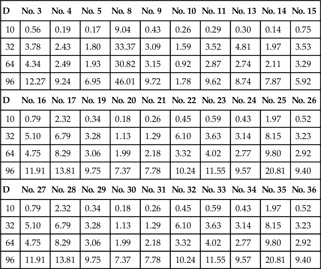
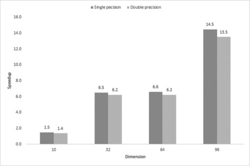
Fig. 12.1 demonstrates the overall speedup for each dimension. On average, cuROB is never slower than its CPU-base CEC’14 benchmark, and speedup of one order of magnitude can be achieved when dimension becomes high. SP is more efficient than DP as far as execution time is concerned.
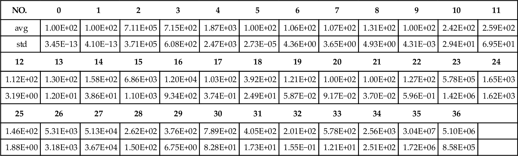
Some preliminary results on standard particle swarm optimization (PSO) are also presented in Table 12.4 as a performance baseline. PSO runs 10 independently for 64 dimension. In each trail, 640,000 function evaluations are conducted.
Table 12.4
Baseline Results for Standard PSO
| NO. | 0 | 1 | 2 | 3 | 4 | 5 | 6 | 7 | 8 | 9 | 10 | 11 |
| avg | 1.00E+02 | 1.00E+02 | 7.11E+05 | 7.15E+02 | 1.87E+03 | 1.00E+02 | 1.06E+02 | 1.07E+02 | 1.31E+02 | 1.00E+02 | 2.42E+02 | 2.59E+02 |
| std | 3.45E−13 | 4.10E−13 | 3.71E+05 | 6.08E+02 | 2.47E+03 | 2.73E−05 | 4.36E+00 | 3.65E+00 | 4.93E+00 | 4.31E−03 | 2.94E+01 | 6.95E+01 |
| 12 | 13 | 14 | 15 | 16 | 17 | 18 | 19 | 20 | 21 | 22 | 23 | 24 |
| 1.12E+02 | 1.30E+02 | 1.58E+02 | 6.86E+03 | 1.20E+04 | 1.03E+02 | 3.92E+02 | 1.21E+02 | 1.00E+02 | 1.00E+02 | 1.27E+02 | 5.78E+05 | 1.65E+03 |
| 3.19E+00 | 1.20E+01 | 3.86E+01 | 1.10E+03 | 9.34E+02 | 3.74E−01 | 2.49E+01 | 5.87E−02 | 9.17E−02 | 3.70E−02 | 5.96E−01 | 1.42E+06 | 1.62E+03 |
| 25 | 26 | 27 | 28 | 29 | 30 | 31 | 32 | 33 | 34 | 35 | 36 | |
| 1.46E+02 | 5.31E+03 | 5.13E+04 | 2.62E+02 | 3.76E+02 | 7.89E+02 | 4.05E+02 | 2.01E+02 | 5.78E+02 | 2.56E+03 | 3.04E+07 | 5.10E+06 | |
| 1.88E+00 | 3.18E+03 | 3.67E+04 | 1.50E+02 | 6.75E+00 | 8.28E+01 | 1.73E+01 | 1.55E−01 | 1.21E+01 | 2.51E+02 | 1.72E+06 | 8.58E+05 |
12.3 Unimodal Functions
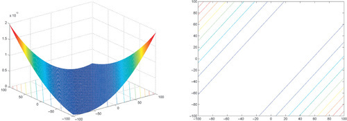
12.3.1 Shifted and Rotated Sphere Function
where z = R(x − xopt).
Properties: Unimodal; Nonseparable; Highly symmetric, in particular rotationally invariant.
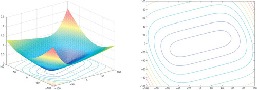
12.3.2 Shifted and Rotated Ellipsoid Function
where z = R(x − xopt).
Properties: Unimodal; Nonseparable.
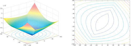
12.3.3 Shifted and Rotated High-Conditioned Elliptic Function
where z = R(x − xopt).
Properties: Unimodal; Nonseparable; Quadratic ill-conditioned; Smooth local irregularities.
12.3.4 Shifted and Rotated Discus Function

where z = R(x − xopt).
Properties: Unimodal; Nonseparable; Smooth local irregularities; With One sensitive direction.
12.3.5 Shifted and Rotated Bent Cigar Function

where z = R(x − xopt).
Properties: Unimodal; Nonseparable; Optimum located in a smooth but very narrow valley.
12.3.6 Shifted and Rotated Different Powers Function
where z = R(0.01(x − xopt)).
Properties: Unimodal; Nonseparable; Sensitivities of the zi variables are different.
12.3.7 Shifted and Rotated Sharp Valley Function
where z = R(x − xopt).
Properties: Unimodal; Nonseparable; Global optimum located in a sharp (non-differentiable) ridge.
12.4 Basic Multimodal Functions
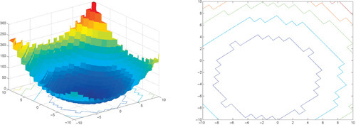
12.4.1 Shifted and Rotated Step Function
where z = R(x − xopt).
Properties: Many Plateaus of different sizes; Nonseparable.
12.4.2 Shifted and Rotated Weierstrass Function
where a = 0.5, b = 3, kmax = 20, z = R(0.005 · (x − xopt)).
Properties: Multimodal; Nonseparable; Continuous everywhere but only differentiable on a set of points.
12.4.3 Shifted and Rotated Griewank Function

where z = R(6 · (x − xopt)).
Properties: Multimodal; Nonseparable; With many regularly distributed local optima.
12.4.4 Shifted Rastrigin Function
where z = 0.0512 · (x − xopt).
Properties: Multimodal; Separable; With many regularly distributed local optima.
12.4.5 Shifted and Rotated Rastrigin Function

where z = R(0.0512 · (x − xopt)).
Properties: Multimodal; Nonseparable; With many regularly distributed local optima.
12.4.6 Shifted Rotated Schaffer’s F7 Function
where ![]() , z = R(x − xopt).
, z = R(x − xopt).
Properties: Multimodal; Nonseparable.
12.4.7 Expanded Griewank Plus Rosenbrock Function
where z = R(0.05 · (x − xopt)) + 1.
Properties: Multimodal; Nonseparable.
12.4.8 Shifted and Rotated Rosenbrock Function
where z = R(0.02048 · (x − xopt)) + 1.
Properties: Multimodal; Nonseparable; With a long, narrow, parabolic shaped flat valley from local optima to global optima.
12.4.9 Shifted Modified Schwefel Function


where z = 10 · (x − xopt).
Properties: Multimodal; Separable; Having many local optima with the second better local optima far from the global optima.
12.4.10 Shifted Rotated Modified Schwefel Function

where z = R(10 · (x − xopt)) and g1(·) is defined as Eq. (12.17).
Properties: Multimodal; Nonseparable; Having many local optima with the second better local optima far from the global optima.
12.4.11 Shifted Rotated Katsuura Function

where z = R(0.05 · (x − xopt)).
Properties: Multimodal; Nonseparable; Continuous everywhere but differentiable nowhere.
12.4.12 Shifted and Rotated Lunacek Bi-Rastrigin Function

where z = R(0.1 · (x − xopt) + 2.5 * 1), μ1 = 2.5, μ2 = −2.5, d = 1, s = 0.9.
Properties: Multimodal; Nonseparable; With two funnel around μ11 and μ21.
12.4.13 Shifted and Rotated Ackley Function
where z = R(x − xopt).
Properties: Multimodal; Nonseparable; Having many local optima with the global optima located in a very small basin.
12.4.14 Shifted Rotated HappyCat Function
where z = R(0.05 · (x − xopt)) − 1.
Properties: Multimodal; Nonseparable; Global optima located in curved narrow valley.
12.4.15 Shifted Rotated HGBat Function
where z = R(0.05 · (x − xopt)) − 1.
Properties: Multimodal; Nonseparable; Global optima located in curved narrow valley.
12.4.16 Expanded Schaffer’s F6 Function

where z = R(x − xopt).
Properties: Multimodal; Nonseparable.
12.5 Hybrid Functions
Hybrid functions are created according to [109]. For each hybrid function, the variables are randomly divided into subcomponents and different basic functions (unimodal and multimodal) are used for different subcomponents, as depicted in Eq. (12.25)

where F(·) is the constructed hybrid function, Gi(·) is the ith basic function used, and N is the number of basic functions. zi is constructed as follows:
where S is a permutation of (1 : D), such that z = [z1, z2,…, zN] forms the transformed vector and ni, i = 1,…, N, are the dimensions of the basic functions, which is derived as Eq. (12.26)

where pi is used to control the percentage of each basic functions.
12.5.1 Hybrid Function 1
• p =[0.3, 0.3, 0.4]
• G1: Modified Schwefel’s Function
• G2: Rastrigin Function
• G3: High Conditioned Elliptic Function
12.5.2 Hybrid Function 2
• p =[0.3, 0.3, 0.4]
• G1: Bent Cigar Function
• G2: HGBat Function
• G3: Rastrigin Function
12.5.3 Hybrid Function 3
• p =[0.2, 0.2, 0.3, 0.3]
• G1: Griewank Function
• G2: Weierstrass Function
• G3: Rosenbrock Function
• G4: Expanded Scaffer’s F6 Function
12.5.4 Hybrid Function 4
• p =[0.2, 0.2, 0.3, 0.3]
• G1: HGBat Function
• G2: Discus Function
• G3: Expanded Griewank plus Rosenbrock Function
• G4: Rastrigin Function
12.5.5 Hybrid Function 5
• p =[0.1, 0.2, 0.2, 0.2, 0.3]
• G1: Expanded Scaffer’s F6 Function
• G2: HGBat Function
• G3: Rosenbrock Function
• G4: Modified Schwefel’s Function
• G5: High Conditioned Elliptic Function
12.5.6 Hybrid Function 6
• p =[0.1, 0.2, 0.2, 0.2, 0.3]
• G1: Katsuura Function
• G2: HappyCat Function
• G3: Expanded Griewank plus Rosenbrock Function
• G4: Modified Schwefel’s Function
• G5: Ackley Function
12.6 Composition Functions
Composition functions are constructed in the same manner as in [110, 109]
where
• F(·): the constructed composition function
• Gi(·): ith basic function
• N: number of basic functions used
• biasi: define which optimum is the global optimum
• σi: control Gi(·)’s coverage range, a small σi gives a narrow range for Gi(·)
• λi: control Gi(·)’s height
• ωi: weighted value for Gi(·), calculated as follows:
where xopt,i represents the optimum position for Gi(·). Then normalize wi to get ![]() .
.
When x = xopt,i, ![]() , such that F(x) = biasi + fopt,i.
, such that F(x) = biasi + fopt,i.
The constructed functions are multimodal and nonseparable and merge the properties of the subfunctions better and maintains continuity around the global/local optima. The local optimum which has the smallest bias value is the global optimum. The optimum of the third basic function is set to the origin as a trip in order to test the algorithms’ tendency to converge to the search center.
Note that the landscape not only changes along with the selection of basic function, but the optima and σ and λ can effect it greatly.
12.6.1 Composition Function 1
• σ =[10, 20, 30, 40, 50]
• λ = [1e − 10, 1e − 6, 1e − 26, 1e − 6, 1e − 6]
• bias = [0, 100, 200, 300, 400]
• G1: Rotated Rosenbrock Function
• G2: High Conditioned Elliptic Function
• G3: Rotated Bent Cigar Function
• G4: Rotated Discus Function
• G5: High Conditioned Elliptic Function
12.6.2 Composition Function 2
• σ = [15, 15, 15]
• λ = [1, 1, 1]
• bias = [0, 100, 200]
• G1: Expanded Schwefel Function
• G2: Rotated Rstrigin Function
• G3: Rotated HGBat Function
12.6.3 Composition Function 3
• σ = [20, 50, 40]
• λ = [0.25, 1, 1e − 7]
• bias = [0, 100, 200]
• G1: Rotated Schwefel Function
• G2: Rotated Rastrigin Function
• G3: Rotated High Conditioned Elliptic Function
12.6.4 Composition Function 4
• σ = [20, 15, 10, 10, 40]
• λ = [2.5e − 2, 0.1, 1e − 8, 0.25, 1]
• bias = [0, 100, 200, 300, 400]
• G1: Rotated Schwefel Function
• G2: Rotated HappyCat Function
• G3: Rotated High Conditioned Elliptic Function
• G4: Rotated Weierstrass Function
• G5: Rotated Griewank Function
12.6.5 Composition Function 5
• σ = [15, 15, 15, 15, 15]
• λ = [10, 10, 2.5, 2.5, 1e − 6]
• bias = [0, 100, 200, 300, 400]
• G1: Rotated HGBat Function
• G2: Rotated Rastrigin Function
• G5: Rotated Schwefel Function
• G4: Rotated Weierstrass Function
• G3: Rotated High Conditioned Elliptic Function
12.6.6 Composition Function 6
• σ = [10, 20, 30, 40, 50]
• λ = [2.5, 10, 2.5, 5e − 4, 1e − 6]
• bias = [0, 100, 200, 300, 400]
• G1: Rotated Expanded Griewank plus Rosenbrock Function
• G2: Rotated HappyCat Function
• G3: Rotated Schwefel Function
• G4: Rotated Expanded Scaffer’s F6 Function
• G5: High Conditioned Elliptic Function
12.6.7 Composition Function 7
• σ = [10, 30, 50]
• λ = [1, 1, 1]
• bias = [0, 100, 200]
• G1: Hybrid Function 1
• G2: Hybrid Function 2
• G3: Hybrid Function 3
12.6.8 Composition Function 8
• σ = [10, 30, 50]
• λ = [1, 1, 1]
• bias = [0, 100, 200]
• G1: Hybrid Function 4
• G2: Hybrid Function 5
• G3: Hybrid Function 6
12.7 Summary
This chapter describes cuROB, a GPU-based benchmark for real parameter optimization problems. cuROB is very flexible. It supports any dimension within the limit of hardware. Powered by the highly parallelled GPU, cuROB can be very efficient which makes it a handy benchmark for testing high dimension problems.
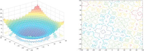
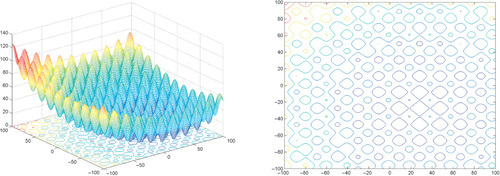
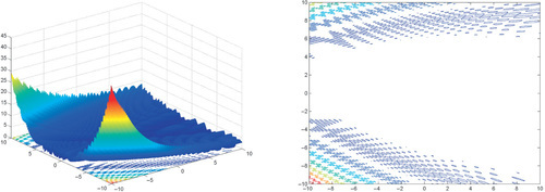
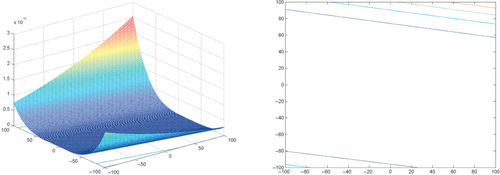
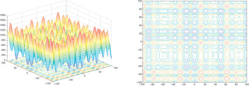
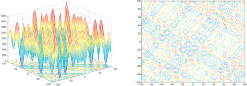
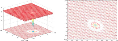
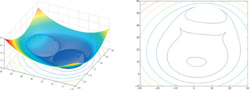
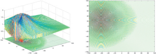
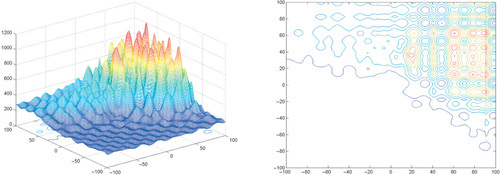
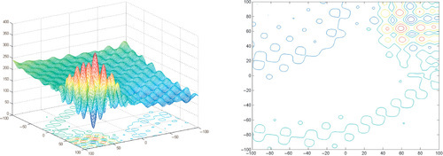
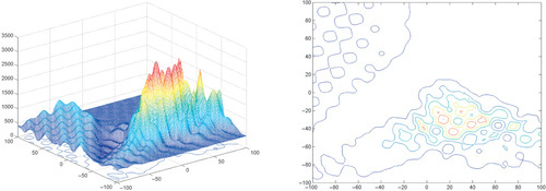
Appendix: Figures for 2D Functions