
It is easy to get caught up in the mystique of artificial intelligence and machine learning when you view the results of an autoencoder or generative adversarial network. The results of these deep learning systems can appear magical and even show signs of actual intelligence. Unfortunately, the truth is far different and even challenges our perception of intelligence.
As our knowledge of AI advances, we often set the bar higher as to what systems demonstrate intelligence. Deep learning is one of those systems that many now view as a mathematical process (machine learning) rather than actual AI. In this book, we won’t debate if DL is AI or just machine learning. Instead, we will focus on why understanding the math of DL is important.
To build generators that work, we need to understand that deep learning systems are nothing more than really good function solvers. While that may dissolve some of their mystique, it will allow us to understand how to manipulate generators to do our bidding.
In this chapter, we take a closer look at how deep learning systems learn and indeed what they are learning. We then advance to understanding variability and how DL can learn the variability of data. From there we use that knowledge to build a variational autoencoder (VAE). Then we learn how to explore the variability to tune the VAE generator. Extending that knowledge, we move on to building and understanding a conditional GAN (CGAN). We finish the chapter using the CGAN to generate pictures of food.
Understanding what deep learning learns
Building a variational autoencoder
Learning distributions with the VAE
Variability and exploring the latent space
It is recommended that you have reviewed the material in Chapters 1–2 before reading this chapter. You may also find it helpful to review the math concepts of probability statistics and calculus. Don’t feel you need to be proficient in calculus; just understand the basic concepts. In the next section, we take a closer look at the math of deep learning.
Understanding What Deep Learning Learns
The math of deep learning is by no means trivial and in many ways was a major hurdle the technology struggled with for decades. It wasn’t until the development of automatic differentiation that deep learning really evolved. Before that, people would spend hours tuning the math for just the simplest of networks. Even the simplest of networks we learned in previous chapters could have taken days or weeks to get the math right.
Now, with automatic differentiation and frameworks like PyTorch or TensorFlow, we can build powerful networks in minutes. What is more, we can teach and empower people with deep learning far quicker. You no longer need a PhD to train networks, and in fact it is common for kids in elementary school to employ deep learning experiments.
Unfortunately, with the good also comes the bad. Automatic differentiation allows us to treat a deep learning system as a black box. That means we may lack some subtle understanding for how a network learns, thereby potentially missing obvious problems in our system or worse yet encounter long struggles trying to fix issues we lack the understanding to resolve.
Fortunately, understanding the math of how a deep learning system learns can be greatly simplified. While it may be difficult to explain these concepts to a five-year-old, anyone who can read a graph and a simple equation will likely understand the concepts in the next section.
Deep Learning Function Approximation
Critical to understanding what deep learning does is understanding that a network is just a good function approximator . In fact, simply put, that is all deep learning systems do. They just approximate known or unknown functions well. Now this can be a bit confusing when we think about how neural networks classify, so let’s look at an example.
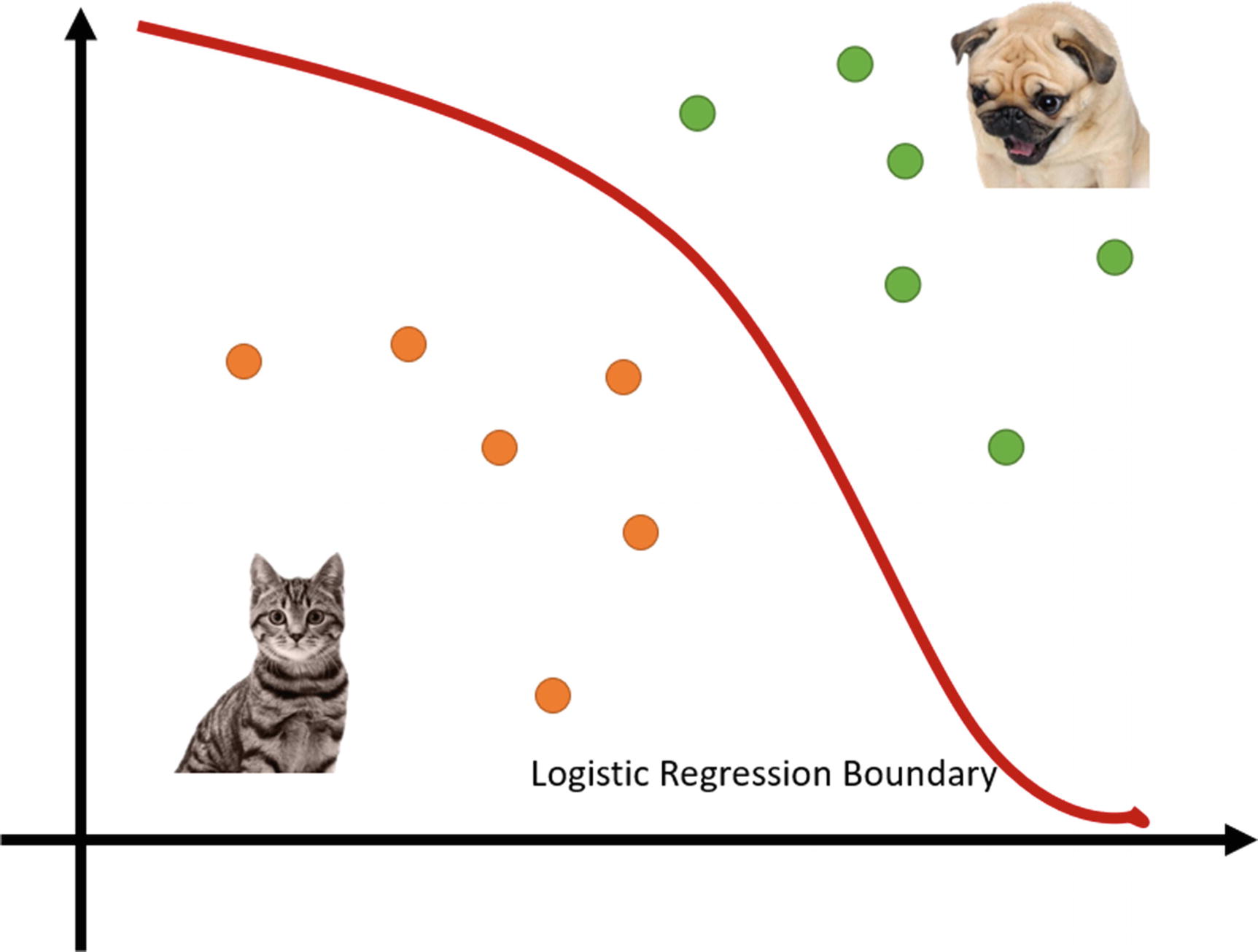
Logistic regression classifying cats and dogs
When a network learns to classify images, it learns the logistics or set of logistic regression functions that break things into classes. While we know there is a set of functions that define the boundary to those classes, in most cases we don’t worry about the exact function. Instead, through training and learning, our deep learning system learns or approximates the function on its own.
To demonstrate how networks do function approximation, we are going to jump into another code example. Exercise 3-1 borrows from a previous regression example, and instead of using data, we can define a known function. Using a known function will demonstrate with certainty how our networks learn.
- 1.
Open the GEN_3_function_approx.ipynb notebook from the GitHub project site. If you are unsure how, then consult Appendix B.
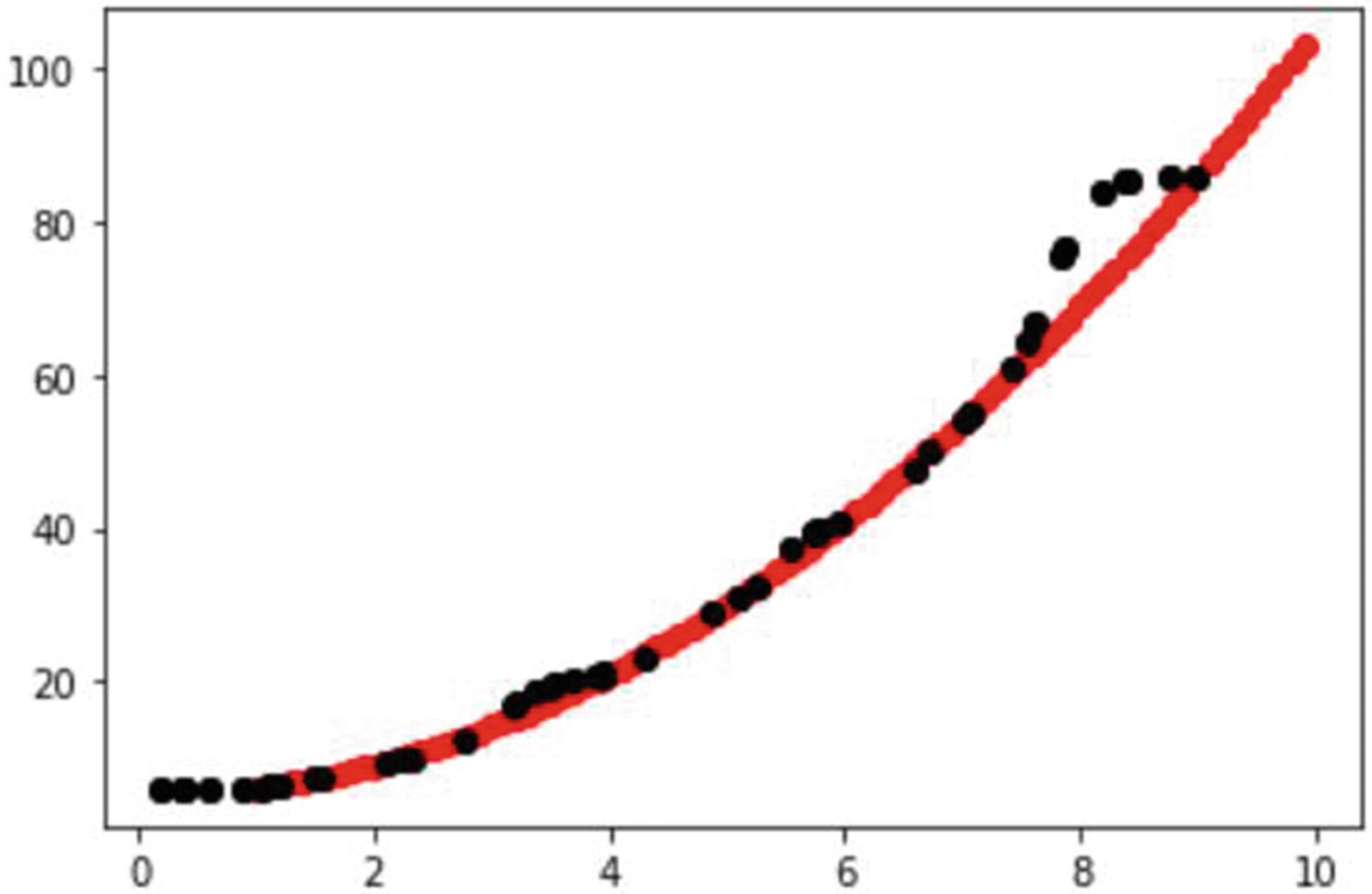
- 2.Run the whole notebook by selecting Runtime ➤ Run all. Then look at the top cells, which define a simple function that we will approximate here:def function(X):return X * X + 5.X = np.array([[1.],[2.],[3.],[4.],[5.],[6.],[7.],[8.],[9.],[10.]])y = function(X)inputs = X.shape[1]y = y.reshape(-1, 1)plt.plot(X, y, 'o', color='black')
- 3.
The function function defines a parabolic equation we will train our network on. In the next cell, you can see how we set up hard-coded X inputs 1–10 that we use to define our learned outputs, y. Notice how we can simply feed the set of inputs X into the function to output our labels or learned values, which are labeled y.
- 4.
Figure 3-2 shows the plotted output of the equation using a sample set of inputs (1–10). This is the equation we want our network to learn how to approximate.
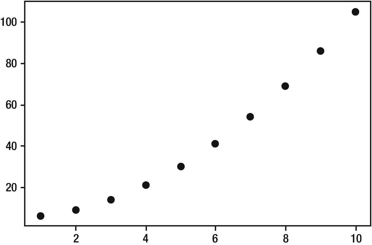
Plotted output of equation values
- 5.We have already reviewed most of the remaining code in previous chapters. Our focus now will be on identifying slight differences. Notice how we still break our input data into training and testing splits with the following:X_train, X_test, y_train, y_test = train_test_split(X, y, test_size=0.2, random_state=0)num_train = X_train.shape[0]X_train[:2], y_train[:2]num_train
- 6.
With only 10 input points, it may seem like a silly step to break the data up into 8/2 points, respectively. However, even when tuning to a known function, it can help validate our results, so we still like to do validation/test splits.
- 7.The only other change to this notebook is another step of validation we do at the end with the following code:X_a = torch.rand(25,1).clone() * 9y_a = net(X_a)y_a = y_a.detach().numpy()plt.plot(X_a, y_a, 'o', color='black')
- 8.
This section of code creates 25 random values using torch.rand. Since the values are from 0–1, we multiply the output by 9 to scale the values from 0–9. We then run the values X_a through the network net and plot the output shown in Figure 3-3.
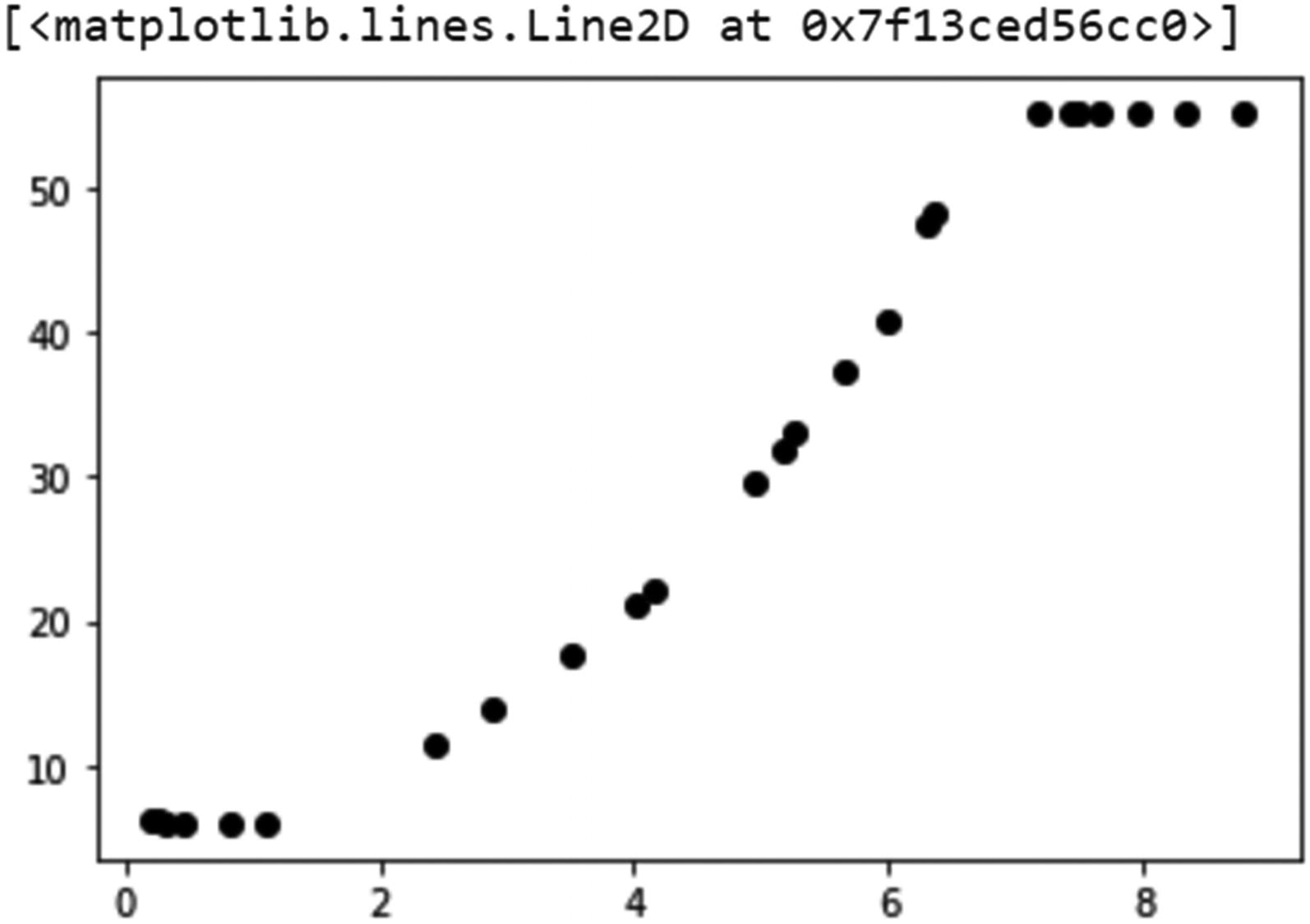
Plotted output of test results on trained network
- 9.
Notice in Figure 3-3 how the network is excellent at approximating the middle values of our known function. However, you can see that the network struggles at the bottom (close to X of 0) and the top end. You can see that the network has greater difficulty approximating the boundaries. Yet it still does very well matching the function’s middle values.
What we just demonstrated is how a simple network can learn to approximate a function. However, we did notice how the network still struggled to approximate the boundaries, and we need to understand why that is.
Part of the problem is the limited amount of data we used to train the network. After all, we used only 10 points. However, the function approximation through the center is very good compared to what happens at the ends. So, why is that?
Simply put, a deep learning system can approximate well to a known or unknown equation within the bounds of the known data or limits of the equation. In our last example, we used data values from 0–10, with bounds of 0 and 10. Yet we see from Figure 3-3 that the function approximation falls down around an input of X=7 or so. As well, on the lower bounds we can see an issue when X<1.
The reason for these inconsistencies is not about the data or indeed the limits to the data but rather the calculus itself. Remember our discussion about auto-differentiation with calculus in Chapter 2? Now the problem isn’t the auto-part of differentiation but rather the differentiation itself.
Calculus helps us to understand the rate of change in an equation or function. This is useful for everything from launching spaceships to building better buildings and of course deep learning. It is also important for us to understand why calculus is used to approximate the functions in deep learning, which is covered in the next section.
The Limitations of Calculus
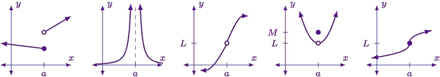
Examples of discontinuous functions
In generative modeling, you can think of a discontinuity as a gap or vacuum in the data. Now don’t confuse a gap in this context with space or distance. We use the term gap here to refer to a break where nothing in the function has any sample values. The term space or latent space or hidden space is used to define the unknown area in a continuous set of data.
Generally, when we see black regions in generated output, that represents a problem with limits or discontinuities in the input data.
Understanding the difference between continuous and discontinuous data will take some time, and sometimes it may not be so obvious. The key takeaway here is to understand that function approximation has limits, and those limits are often defined by the data itself, sometimes requiring a network to approximate a continuous function over discontinuous data.
Now, getting back to limits, let’s understand how limits can affect how a network learns or approximates to data. In our exercise example, our network had limits of 1 and 10. If we refer to Figure 3-3, we can see that our function flattens at X<1, which makes sense considering the limit of 1. This means our network just limits the function approximation to y=5 when X is less than 0.
What is not so obvious, however, is why our function approximation fails on values greater than 7 when the limit was 10. To understand why this issue arises, we need to understand how deep learning uses calculus to approximate functions, which is covered in the next section.
Deep Learning Hill Climbing
At the heart of any deep mathematical concept there is always a grounded intuition that explains the why. Unfortunately, most classic mathematics courses often miss explaining the why. Instead, they rely on the student to uncover the intuition on their own through performing proofs or regurgitating equations. This is something that works well for budding mathematicians but tends to overwhelm everyone else. For that reason, we will always focus more on the why of the math rather than the specific how.
Calculus is a tool we use in deep learning systems to balance the weights/parameters of a network. Recall that calculus works by understanding the rate of change of a system. In deep learning, calculus allows us to determine how much change and to where we need to adjust the weights in a network.
Calculus and gradient optimization or gradient descent is not the only tool we can use to find the weights in a network. It is currently the most efficient, but deep learning systems have and continue to use other machine learning methods. If you are interested in learning more, Google deep learning PSO or deep learning GA.
Figure 3-4 shows a one-dimensional function with a ball at position 1. We can think of the goal of a deep learning system as guiding that ball over the function. Further yet, we want the ball to be able to follow that function as close as possible. The better that ball is able to follow the function path, the better our networks will predict or generate content.
Notice that in Figure 3-4 we are moving the ball an amount calculated through automatic differentiation and our optimization method multiplied by the learning rate (alpha). This is labeled “Gradient X alpha” in the figure. The amount of gradient can be altered by selecting different optimization methods and/or tuning the hyperparameters. Tuning the optimizer, be it stochastic gradient descent or Adam, is something we will cover later.

Deep learning hill climbing

Adjusting the learning rate
The primary takeaway from this is that the learning rate is often our most sensitive hyperparameter when mapping to functions. Learning rate, or alpha, is almost always the first to tune and understand for your network. Alpha is also the key to tuning how quickly a network will train. When alpha is too large, the network will overshoot the function. Conversely, keeping alpha very small allows the ball to learn the function well. However, this can come at great cost of computing performance.
Consider a learning rate of .001 compared to a value of .00001. Say we can train a network with the smaller rate in, say, 10 minutes. The smaller rate, being 100 times smaller, would likely take 100 times longer due to the increase in training iterations, increasing training times to 10 × 100 = 1000 minutes, or more than 16 hours. This is all from a smaller but unfortunately less efficient learning rate.
To demonstrate this key concept further, let’s look at another example. Exercise 3-2 shows how we will tune the alpha (learning rate) to better approximate the function in our previous exercise.
- 1.
Open the GEN_3_learning_rate.ipynb notebook from the GitHub project site. If you are unsure how, then consult Appendix B.
- 2.Run the whole notebook by selecting Runtime ➤ Run all. Notice that where we define the optimizer, as shown in the following code, is where we set the learning rate lr.loss_fn = nn.MSELoss()optimizer = torch.optim.Adam(net.parameters(), lr = .001)
- 3.
In our previous example of GEN_3_function_approx.ipynb, our learning rate was .025, a value that was on the cusp of being able to correctly map the function.
- 4.
Our goal here is to find the learning rate that will allow the network to map 100 percent to the function or close to it.
- 5.
Change the learning rate lr in the previous block of code and rerun the entire notebook by selecting Runtime ➤ Run all.
- 6.
See if you can tune the lr value to match or approximate Figure 3-7. What happens if you make the learning rate really small?
- 7.If your network completes training before finding the function, this is easily fixed by increasing the number of epochs. Change num_epochs to something larger and see what results this has.num_epochs = 8000y_train_t = torch.from_numpy(y_train).clone().reshape(-1, 1)
- 8.
Attempt to find the smallest number of epochs and the greatest learning rate that will train the network to match the function x2 + 5.
- 9.
If you are feeling more advanced, try altering the number of neurons in each layer or altering the network itself.

Better approximation to the function x2 + 5?
As you worked through the previous exercise, it may have occurred to you that there may be limitations to the network itself and the data. In fact, that is exactly the case in the exercise. For this particular example, the network attempts to overfit the data. We will look at how to resolve both over- and underfitting in the next section.
Over- and Underfitting
Oftentimes when newcomers design networks, their first assumption is that having more neurons means better results. Unfortunately, this is rarely the case for a number of reasons that we will understand in later chapters. For now, we want to focus on how the network size itself can overfit or underfit to the function.
You may often hear deep learners mention their network is over- or underfitting to the data. What they really mean is that the network is over- or underfitting to the function that matches or categorizes that data.
Trained model plotted against actual function x2 + 5
Think back to our previous exercise and our attempts to approximate to the function x2 + 5. Our first couple of attempts used a set number of data points from 1 to 10. We fed those data points into the function to generate y outputs. This generated our set of trainable data, which we then broke up into training and testing splits.

Plot of input dataset from Exercise 3-1 and Exercise 3-2
That means when our model goes to approximate the function x2 + 5, it has large areas between data. We call these areas the latent or hidden space. Again, this is not to be confused with a gap, chasm, or vacuum in the data. This hidden space in the data represents an area of the function missing any actual training data. That means the network must approximate values between these data points.
As it turns out, a big part of generative modeling is understanding how to extract results from this latent space, as we will see throughout this book. It’s not unlike how we tried to extract the results of our previous function approximation exercise. Our previous assumption may have been to reduce the number of training points, but as we can see now, this increases the size of the latent space, causing our model to overfit to the function.
Overfitting is caused when a model approximates to a function but wrongly fills or approximates the latent space. In our previous function approximation examples, this was clearly the case, which was caused by two problems. The first was the lack of data, which caused the network to estimate large areas of latent space. The second was the size of our network, which had too much power to estimate the space in data. So, it essentially made up values, which can be a problem.
When a network is large, it has a lot of power, in this case too much power. Large networks can memorize data of all forms including images or video. This may be useful for networks scoped to specific data, but in generative modeling as well as most other machine learning disciplines, our goal is always to generalize.
Generalizing is always a goal we will undertake when building models. That means the data we feed into the model needs to be well distributed. Well-distributed data provides us with even latent space between data. In our previous example, our data was distributed into 10 bins, with values from 1–10. However, as we can see, our data was not distributed well enough.
Generalizing also means that our network should be only the size it needs, no more or less. If our network is too large, it will tend to overfit or fill in those latent space with incorrect values. Likewise, networks that are too small will underfit. Underfitting is often a consequence of too large of gaps or latent space in a model.

A linear model trying to fit to the function x2 + 5
To understand this in a tangible manner, our next exercise will focus on how we create models that over- and underfit to a set of function data. We will continue to use the base of our previous exercise, but this time we will modify some details to understand the problem better; see Exercise 3-3.
- 1.
Open the GEN_3_over_under.ipynb notebook from the GitHub project site. If you are unsure how, then consult Appendix B.
- 2.Run the whole notebook by selecting Runtime ➤ Run all. Notice how we changed the inputs (X,y) in the block just before the output plot, as shown here:data_step = .1X = np.reshape(np.arange(1,10, data_step), (-1, 1))y = function(X)inputs = X.shape[1]plt.plot(X, y, 'o', color='red')
- 3.
In the previous block of code, we alter the NumPy calls so that we autogenerate our array using np.arange. The arange function takes as input the start and end and the step size. We use a new hyperparameter called data_step to set the distance in latent space. Using a step size of .1 allows us to create 10 times the number of data points we previously used, thus greatly reducing those latent spaces.
- 4.Next, notice in this example how the hyperparameters of learning rate (lr) and the number of epochs (num_epochs) have been altered:optimizer = torch.optim.Adam(net.parameters(), lr = .01)num_epochs = 1000
- 5.The network design has also been altered by removing a layer and putting in another hyperparameter called neurons.neurons = 20torch.set_default_dtype(torch.float64)net = nn.Sequential(nn.Linear(inputs, neurons, bias = True), nn.ReLU(),nn.Linear(neurons, neurons, bias = True), nn.Sigmoid(),nn.Linear(neurons, 1))
- 6.
The neurons hyperparameter allows us to quickly alter the network size, allowing us to reduce the number of neurons to either over- or underfit the network.
- 7.
Try adjusting just the two hyperparameters, data_step and neurons, to see what effect this has on over- or underfitting the model. Keep in mind that larger and complex models generally require more training iterations, num_epochs. This in turn means you may want to alter the learning rate lr, as well.
- 8.
Now try to find the smallest network, the least number of neurons, that can learn the function the quickest, with fewer num_epochs. Feel free to adjust the learning rate (lr) and data_step as you need.
- 9.
Finally, set data_step to a high value like 1.0 and then see what effect altering the neurons has. Do you need to increase or decrease the number of neurons?
The intention of the previous exercise was to demonstrate how our networks can over- and underfit the function that maps to our data. In this simple example, we could see quick and explicit feedback for what each of our hyperparameters did, allowing us to understand how a network can over- or underfit.
As we progress through this book and use more complex forms of data, like images, over- and underfitting often becomes less obvious. Fortunately, there are several clues that can help us identify these types of problems that we explore as we progress to those exercises.
One key element we didn’t cover and can cause a lot of over/underfitting issues is data distribution. In the examples, the data was uniformly distributed across a range of values. This is rarely something we see in the real world.
For example, assume you had a dataset of 30,000 animal images (10,000 cats, 15,000 of dogs, and 5,000 birds) that you wanted to classify into cats, dogs, and birds. The problem is your data is not evenly distributed. You have more pictures of dogs, and hence your model will overestimate or memorize dogs. Instead, what we should do is reduce the number of cat and dog images to 5,000 to match the number of bird images. You could still argue that the cat and dog are more visually similar than a bird, thus potentially influencing your results.
We use and understand how data is distributed in several ways in generative modeling. It is in fact a foundation of many of the methods. In the next section, we will understand why data distributions are important to the variational autoencoder.
Building a Variational Autoencoder
In our previous example exercises, we explored how networks perform function approximation and discovered the latent space at discrete intervals. We found that by increasing our amount of data sampling intervals we could reduce our unknown latent space and improve our model training. This is a technique that works well for simplistic functions but does not scale to more complex problems.
A better approach to understanding our problem and the data itself is with statistics. Statistics allows us to understand the model and latent space in the data. In turn, statistics can provide us with a summary or overview of the models and the way we generate new data.
Statistics are fundamental to data science, deep learning, and generative modeling. In data science we use statistics to make decisions on what data to use. For deep learning, statistics are used to measure a model’s efficiency, while generative modeling uses statistics to understand what the model is learning.
Now before we jump into the statistics of generative modeling and understanding latent spaces, it would be helpful to look at a working example. This example also can take a while to train, so while it does, you can read up on the theory in the next section.
In our next exercise, we are going to dive in and build a variational autoencoder (VAE). A VAE is like an autoencoder in structure and function except in how it learns that encoding part. Remember in an AE, the model learns how to encode a latent representation of the data before decoding it back to the original. In a VAE, the model learns how the latent encoding is distributed. We won’t worry about understanding the distributed part just yet but instead jump in and see how the code works in Exercise 3-4.
- 1.
Open the GEN_3_conv_VAE.ipynb notebook from the GitHub project site.
- 2.Run the whole notebook by selecting Runtime ➤ Run all. Just below the first import cell, you will notice a cell checking for the device type, as shown in the following code:device = torch.device('cuda' if torch.cuda.is_available() else 'cpu')device
- 3.For this notebook and all future notebooks, we will be configuring the runtime to use a GPU. Figure 3-11 shows the runtime type accessible from the menu by selecting Runtime ➤ Change runtime type.
 Figure 3-11
Changing the runtime type on a Colab notebook
- 4.Since we covered the next few sections of data handling code before, we will jump down to the cell that defines the ConvVAE class and the __init__ function.class ConvVAE(nn.Module):def __init__(self, image_channels=3, h_dim=1024, z_dim=32):super(ConvVAE, self).__init__()self.encoder = nn.Sequential(nn.Conv2d(image_channels, 32, kernel_size=4, stride=2),nn.ReLU(),nn.Conv2d(32, 64, kernel_size=4, stride=2),nn.ReLU(),nn.Conv2d(64, 128, kernel_size=4, stride=2),nn.ReLU(),nn.Conv2d(128, 256, kernel_size=4, stride=2),nn.ReLU(),Flatten())self.fc1 = nn.Linear(h_dim, z_dim)self.fc2 = nn.Linear(h_dim, z_dim)self.fc3 = nn.Linear(z_dim, h_dim)self.decoder = nn.Sequential(UnFlatten(),nn.ConvTranspose2d(h_dim, 128, kernel_size=5, stride=2),nn.ReLU(),nn.ConvTranspose2d(128, 64, kernel_size=5, stride=2),nn.ReLU(),nn.ConvTranspose2d(64, 32, kernel_size=6, stride=2),nn.ReLU(),nn.ConvTranspose2d(32, image_channels, kernel_size=6, stride=2),nn.Sigmoid(),)
- 5.
This code is like the convolutional autoencoder we looked at before. The key difference here is the use of the three nn.Linear layers that now are responsible for learning the middle encoding distribution. Previously we defined a discrete data size as our learning representation. Have some patience: we will talk more about learning distributions later.
- 6.Jump over the remaining functions in the ConvVAE class and down to the block of code where the optimizer is defined.optimizer = torch.optim.Adam(model.parameters(), lr=learning_rate)def loss_fn(recon_x, x, mu, logvar):BCE = F.binary_cross_entropy(recon_x, x, size_average=False)KLD = -0.5 * torch.mean(1 + logvar - mu.pow(2) - logvar.exp())return BCE + KLD, BCE, KLD
- 7.
We can see in the previous code the definition of a specialize loss function loss_fn. The code in this function is responsible for learning latent encoding distribution. Again, details to come later.
- 8.Finally, we come to the last block of the training code. This section is almost identical to our previous exercises. One key difference to note, however, is the highlighted line starting with images =. This line converts the images from a CPU tensor to a GPU tensor, the difference being where the memory resides and how it is processed. Tensors processed on GPUs can increase performance by more than 100x.for epoch in range(epochs):train_loss = 0.0for data in train_loader:images, labels = dataoptimizer.zero_grad()images = images.to(device)generated, mu, logvar = model(images)loss, bce, kld = loss_fn(generated, images, mu, logvar)loss.backward()optimizer.step()train_loss += loss.item()*images.size(0)train_loss = train_loss/len(train_loader)clear_output()print(f'Epoch: {epoch+1} Training Loss: {train_loss:.3f}')plot_images(generated.cpu().data,labels,16)
- 9.
Keep the notebook training as you continue reading through the next section. Be sure to check back periodically to see how the model progression learns. If you are not happy with the results, keep the model training by running the last cell. Each run of the last cell will add another 100 iterations of training to the model.
You can keep incrementally training your model if the notebook’s runtime is not reset or expires. The runtime can be manually reset in the notebook or Google will expire it for you over time. Google suggests a runtime is good for 12 hours, but several factors appear to affect that. A few can be the number of notebooks you are running, if they are using GPUs and traffic.

Training results of VAE after 1, 50, and 101 iterations
Now that we have seen how a VAE can function, we want to understand how the internal model works and learn the distribution or variation of the data in the next section.
Learning Distributions with the VAE
In a VAE, the model learns by not just understanding a middle or latent space encoding but rather how the encoding itself is distributed. By understanding the distribution or variability of the encoding, we can then learn to map across the latent encoding and generate those hidden spaces.
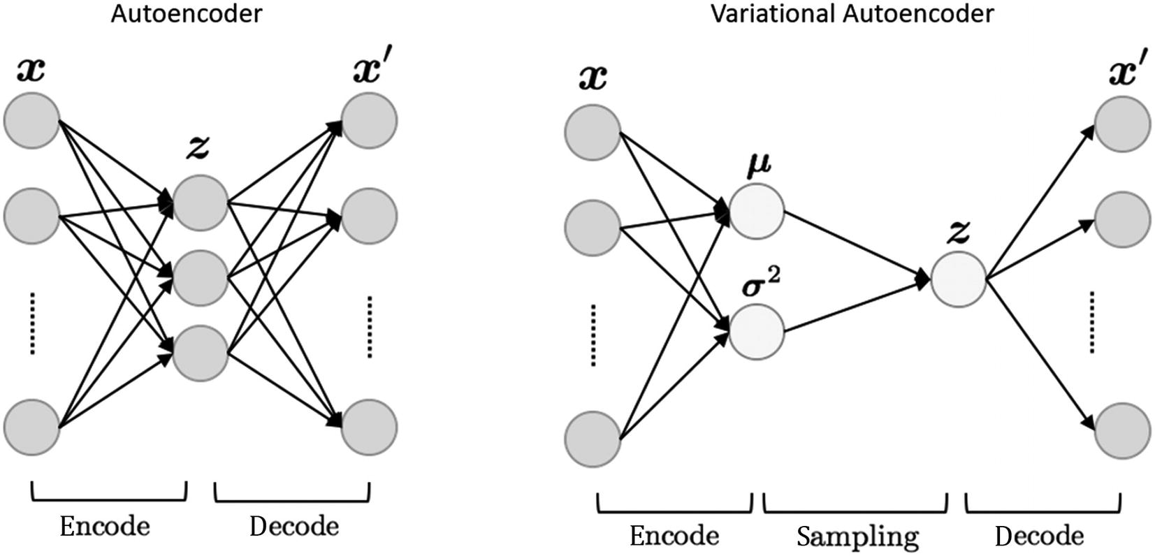
Comparison of AE vs. VAE
The parameters this VAE model learns are the mean (μ) and standard deviation or variance squared (σ2). If you recall from statistics, these are the same parameters we use to define a normal distribution. We often default to the normal distribution, but it is important to understand that data can be distributed in a myriad of ways.

Examples of various distributions
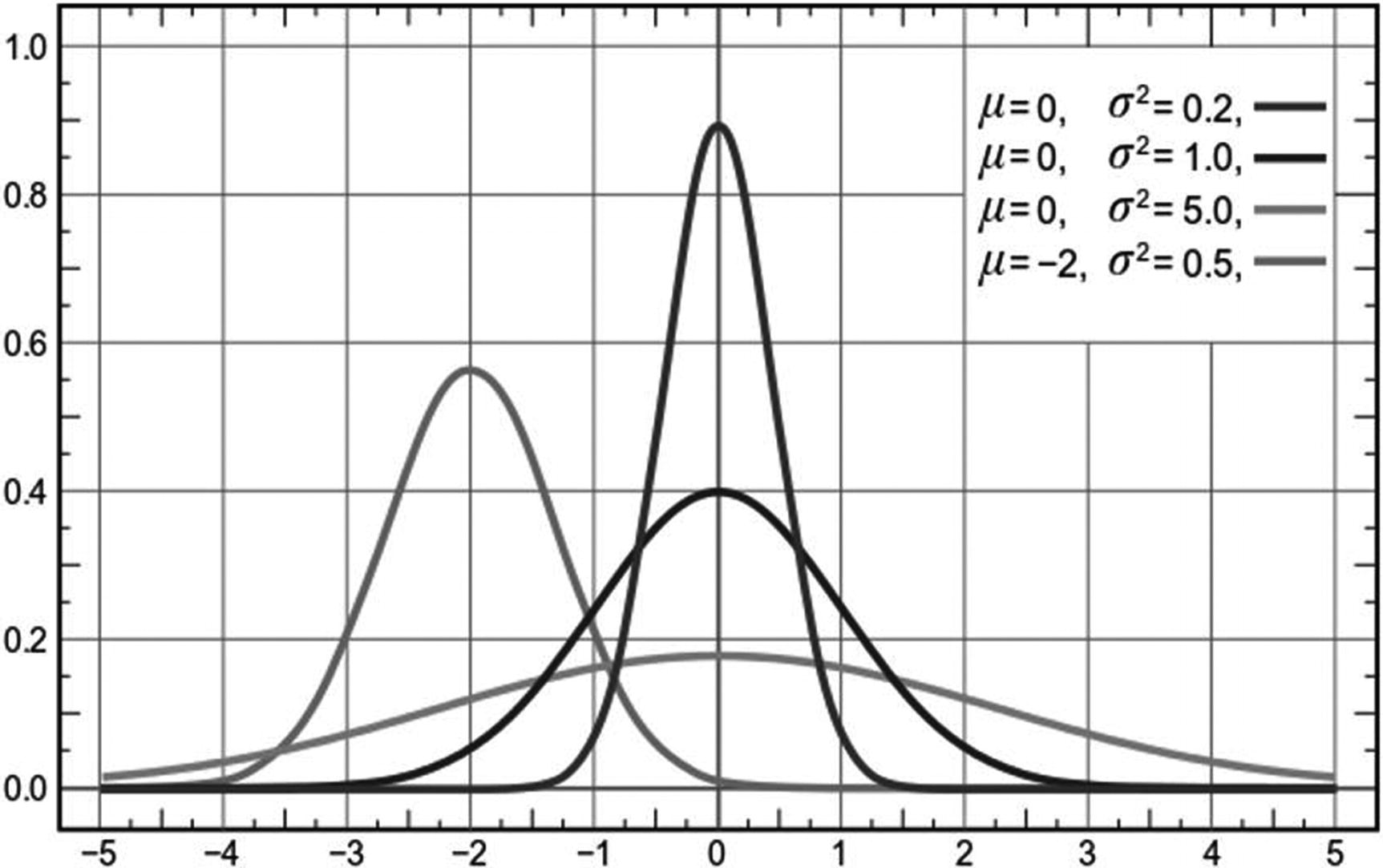
Example of normal distributions modified by μ and σ2
In Figure 3-15 we can see how different variations of μ and σ2 alter the shape of the normal distribution, where the mean always represents the center of the distribution and the standard deviation represents the spread or diversity.
Typically, we use statistics to find how data is distributed or what variability it represents. With a VAE we are still learning what the parameters of the data are, except now the data space we are focusing on becomes the hidden or latent space representation of that data. This has three advantages over trying to learn the entire latent space of a set of training images.
First, by learning the embedding space, the amount of data or dimensions of data can be greatly reduced. This allows our VAE to learn how features are represented in a simpler form, which in turn allows us to model a simple normal distribution. More complex forms of data could require a VAE to model more complex distributions or sets of distributions.
The second advantage provides us with the ability to map or generate from this learned latent space into new output. All we need to do is understand and control those distributional parameters, and we have new novel outputs.
The third advantage (but perhaps less of one) is the confirmation that we can generate output by just learning the input data distribution and converting it into normal parameters. One key architectural difference between an AE and VAE is the sampling operation that takes place in the middle of the model. This operation essentially decouples the encoder and decoder models, providing us with the ability for better reuse and further generative modeling opportunities.
Of course, to understand this better, we need to jump back into another code exercise and see how all this comes together. In the next exercise, we go under the covers of VAE to understand how it learns the distribution or variability of the encoded space; see Exercise 3-5.
- 1.
Open the GEN_3_conv_VAE_latent.ipynb notebook from the GitHub project site.
- 2.
Run the whole notebook by selecting Runtime ➤ Run all.
- 3.Jump down to the class definition code block and the encode and decode functions shown here:def bottleneck(self, h):mu, logvar = self.fc1(h), self.fc2(h)z = self.reparameterize(mu, logvar)return z, mu, logvardef encode(self, x):h = self.encoder(x)z, mu, logvar = self.bottleneck(h)return z, mu, logvardef decode(self, z):z = self.fc3(z)z = self.decoder(z)return zdef forward(self, x):z, mu, logvar = self.encode(x)z = self.decode(z)return z, mu, logvar
- 4.
Notice how the network restricts using the bottleneck function to generate the mu and logvar or variance parameter. Those parameters are then used to sample a z or encoded representation from the distribution. Then in the forward function we can see how encode is used to generate those parameters as well as the sampled z, with z being fed into the decoder as the encoding used to generate new output.
- 5.Next, we will scroll down to the loss_fn again, shown here:def loss_fn(recon_x, x, mu, logvar):BCE = F.binary_cross_entropy(recon_x, x, size_average=False)KLD = -0.5 * torch.mean(1 + logvar - mu.pow(2) - logvar.exp())return BCE + KLD, BCE, KLD
- 6.
The customized loss function in this case is using two methods to measure the divergence between the learned distribution and that observed. The first technique is called binary cross entropy (BCE), which measures the difference in the raw input image and the reconstructed one. It’s is not unlike how we measured loss in a vanilla AE. The second technique is called Kullback Leibler Divergence (KLD) and is used to measure the actual difference in data distributions.
- 7.
Figure 3-16 shows how KLD can be used to measure the difference between two normal distributions. The shaded area represents the divergence between the two distributions. Our goal of calculating the combined loss using BCE and KLD allows us to learn the values of the mean and standard deviation by minimizing this difference in distributions via the loss function.
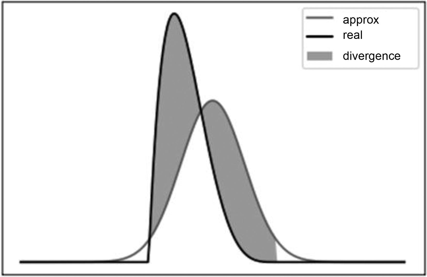
Showing measured divergence between two normal distributions
- 8.
Let the notebook run until it completes at a minimum of 100 epochs. You will want a good model to better understand the next section.
- 9.
The following block is responsible for generating the example output comparison shown in Figure 3-17. In this figure we see the original images used to input into the VAE to generate the output images. Notice how the output is relatively good considering all the VAE learns is to map the data distribution of the input image.

Input images versus output generated images
With the output in Figure 3-17 you can start to appreciate the power of learning the distribution of data in an image. Realize that with each input image the VAE is learning how the data/pixels in the image are being distributed. It then uses that knowledge captured in the learned mean and standard deviation to create a normal distribution that it then uses to randomly sample from. Thus, each of the output images in the VAE reconstruction is randomly sampled from the learned distribution.
The concept of learning how data is distributed, and mapping that to a known or unknown function, is the core of generative modeling with deep learning. We will use this concept repeatedly as we progress through this book. In the next section, we look at how understanding the distribution of data allows us to also manipulate output.
Variability and Exploring the Latent Space
With a trained VAE model, we can begin to explore the latent space of what the model learns. Throughout this chapter we have been working toward understanding what that latent space looks like. Now we are at a position to unfold that latent space and view the contents visually.
The best way to visualize the latent space encodings in a VAE is to visualize the output or the controlled output. We can do that a couple of ways, and in Exercise 3-6 we explore how to search the output space of a learned VAE.
- 1.
Jump to your last and trained version of the GEN_3_conv_VAE_latent.ipynb notebook. If you need to train the notebook again, do so; it can take about up to an hour. We will look at how to save and restore models later, but for now just retrain if you need to.
- 2.At the bottom of this notebook are two code cells that allow us to map the output of the model either randomly or controlled across the latent space distribution parameters, mean, and standard deviation.with torch.no_grad():# sample latent vectors from the normal distributionlatent = torch.randn(60, 1024, device=device)# reconstruct images from the latent vectorsimg_recon = model.decoder(latent)img_recon = img_recon.cpu()fig, ax = plt.subplots(figsize=(20, 20))show_image(torchvision.utils.make_grid(img_recon.data[:100],10,5))plt.show()
- 3.
The first block of code shown earlier generates the sample latent vectors using the torch.randn function to generate 60 vectors of size 1024. We get 1024 from the latent vector size used in our VAE; 1024 is a much larger latent vector than we used when exploring autoencoders, which is to account for the more complicated training dataset. The rest of the code uses model.decoder to use the latent vector as input to generate a new set of images.
- 4.
Figure 3-18 shows the sample output from this last code cell. The output here effectively represents entirely random vectors fed into the decoder part of the VAE to generate output. As you can see, the results are less than spectacular.

Example output from random latent space generation
- 5.The next and last blocks of code demonstrate how we can cycle through the normal distribution parameters to generate not random samples, but samples created from a known distribution. This allows us to understand what the visual area in our model looks like between the data and the latent space.for std in np.arange(.75, 1.5, .1):for mean in np.arange(-2, 3, 1):with torch.no_grad():# sample latent vectors from the normal distributionlatent = torch.normal(mean, std, size=(10, 1024), device=device)# reconstruct images from the latent vectorsimg_recon = model.decoder(latent)img_recon = img_recon.cpu()fig, ax = plt.subplots(figsize=(20, 20))show_image(torchvision.utils.make_grid(img_recon.data[:100],10,5))ax.axis('off')print(mean, std)plt.show()
- 6.
Now instead of generating an entire batch of random images, we generate a strip of 10 images with each update of the std and mean. This allows us to determine the amount of sensitivity in these parameters but also how they visually generate output.
- 7.
Figure 3-19 shows an extracted snippet of the output from the last code cell. Notice how the change to mean and std change the look of the output. Also notice how the model attempts to replicate features it learned. This feature reconstruction is the result of our convolutional layers creating those features. In some cases, you may see recognizable features that belong to specific classes like cats or dogs. See Figure 3-19.
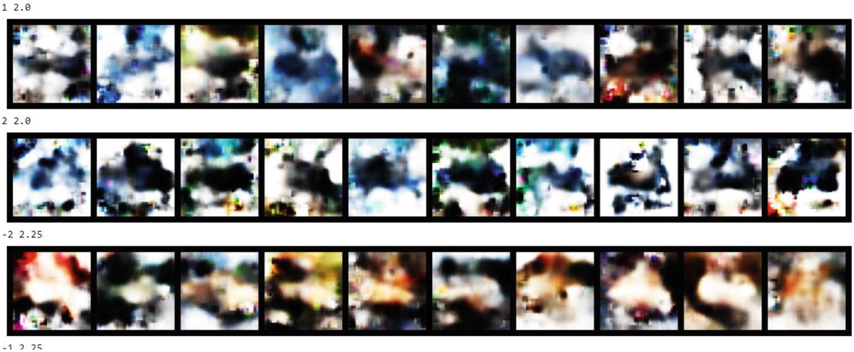
Example output of sample latent space parameters
- 8.
Now that you understand the how a VAE works, try to tune the hyperparameters batch_size, learning_rate, and epochs. Recall what we learned earlier in this chapter.
- 9.
If you are feeling more advanced, try altering the hidden latent vector size h_dim from 1024 to a different number. Also try modifying the z_dim hyperparameter from 32 to 64 or 16. What effect does this have? Hint: the code where you can find those two hyperparameters is shown here:
In the previous exercise, we started to visually explore the latent space in our models. This technique provides us with greater feedback on how well our model trains and what it is training to. We will use techniques like we used in the previous exercise repeatedly throughout this book.
Exploring the latent space in a VAE is useful and provides several insights. Unfortunately, mapping to distributional parameters still very much limits our model’s learning abilities. Fortunately, the model we already explored, the GAN, already learns the latent distribution of data. We will explore more about how GANs do this in the next chapter.
Conclusion
To construct working and practical generative models, we need to understand how deep learning networks learn. We needed to learn how networks approximate to functions and what effect that has on what the network learns. From that we explored in some detail how the various hyperparameters can affect how and what a network learns, further learning how to tune those hyperparameters on toy examples.
Next, we moved from tuning to understanding how hyperparameters can allow us to control the latent or hidden space in our models. Learning to control the size of latent space allowed us to better train the models. Then we advanced to building a variational autoencoder, a model that learns by understanding not just the latent space but distributional parameters that map to that latent space.
Finally, from our knowledge of mapping parameters to the latent space, we could then construct output strictly based on those parameters. This allowed us to see in detail what our model learns and how sensitive it is to the input data. While we didn't look to resolve issues with our model in this chapter, we will certainly look to other systems in the future to improve on it.
In the next chapter, we will revisit GAN and move on to explore its many variations. GANs can be adapted to easily to control the latent space in model generation using several techniques, many of them related to distributional learning. This will allow us to generate content in a more controlled manner.