11
Composing Music with Generative Models
In the preceding chapters, we discussed a number of generative models focused on tasks such as image, text, and video generation. In the contexts of very basic MNIST digit generation to more involved tasks like mimicking Barack Obama, we explored a number of complex works along with their novel contributions, and spent time understanding the nuances of the tasks and datasets involved.
We saw, in the previous chapters on text generation, how improvements in the field of computer vision helped usher in drastic improvements in the NLP domain as well. Similarly, audio is another domain where the cross-pollination of ideas from computer vision and NLP domains has broadened the perspective. Audio generation is not a new field, but thanks to research in the deep learning space, this domain has seen some tremendous improvements in recent years as well.
Audio generation has a number of applications. The most prominent and popular ones nowadays are a series of smart assistants (Google Assistant, Apple Siri, Amazon Alexa, and so on). These virtual assistants not only try to understand natural language queries but also respond in a very human-like voice. Audio generation also finds applications in the field of assistive technologies, where text-to-speech engines are used for reading content onscreen for people with reading disabilities.
Leveraging such technologies in the field of music generation is increasingly being explored as well. The acquisition of AI-based royalty-free music generation service Jukedeck by ByteDance (the parent company of social network TikTok) speaks volumes for this field's potential value and impact.1
In fact, AI-based music generation is a growing trend with a number of competing solutions and research work. Commercial offerings for computer-aided music generation, such as Apple's GarageBand,2 provide a number of easy-to-use interfaces for novices to compose high-quality music tracks with just a few clicks. Researchers on Google's project Magenta3 are pushing the boundaries of music generation to new limits by experimenting with different technologies, tools, and research projects to enable people with little to no knowledge of such complex topics to generate impressive pieces of music on their own.
In this chapter, we will cover different concepts, architectures, and components associated with generative models for audio data. In particular, we will limit our focus to music generation tasks only. We will concentrate on the following topics:
- A brief overview of music representations
- RNN-based music generation
- A simple setup to understand how GANs can be leveraged for music generation
- Polyphonic music generation based on MuseGAN
All code snippets presented in this chapter can be run directly in Google Colab. For reasons of space, import statements for dependencies have not been included, but readers can refer to the GitHub repository for the full code: https://github.com/PacktPublishing/Hands-On-Generative-AI-with-Python-and-TensorFlow-2.
We will begin with an introduction to the task of music generation.
Getting started with music generation
Music generation is an inherently complex and difficult task. Doing so with the help of algorithms (machine learning or otherwise) is even more challenging. Nevertheless, music generation is an interesting area of research with a number of open problems and fascinating works.
In this section, we will build a high-level understanding of this domain and understand a few important and foundational concepts.
Computer-assisted music generation or, more specifically, deep music generation (due to the use of deep learning architectures) is a multi-level learning task composed of score generation and performance generation as its two major components. Let's briefly discuss each of these components:
- Score generation: A score is a symbolic representation of music that can be used/read by humans or systems to produce music. To draw an analogy, we can safely consider the relationship between scores and music to be similar to that between text and speech. Music scores consist of discrete symbols which can effectively convey music. Some works use the term AI Composer to denote models associated with the task of score generation.
- Performance generation: Continuing with the text-speech analogy, performance generation (analogous to speech) is where performers use scores to generate music using their own characteristics of tempo, rhythm, and so on. Models associated with the task of performance generation are sometimes termed AI Performers as well.
We can realize different use cases or tasks based on which component is being targeted. Figure 11.1 highlights a few such tasks that are being researched in the context of music generation:

Figure 11.1: Different components of music generation and associated list of tasks
As shown in the figure, by focusing on score generation alone, we can work toward tasks such as melody generation and melody harmonization, as well as music in-painting (associated with filling in missing or lost information in a piece of music). Apart from the composer and the performer, there is also research being done toward building AI DJs. Similar to human disc jockeys (DJs), AI DJs make use of pre-existing music components to create medleys, mashups, remixes, and even highly personalized playlists.
In the coming sections, we will work mainly toward building our own score generation models or AI Composers. Now that we have a high-level understanding of the overall music generation landscape, let's focus on understanding how music is represented.
Representing music
Music is a work of art that represents mood, rhythm, emotions, and so on. Similar to text, which is a collection of alphabets and grammatical rules, music scores have their own notation and set of rules. In the previous chapters, we discussed how textual data is first transformed into usable vector form before it can be leveraged for any NLP task. We would need to do something similar in the case of music as well.
Music representation can be categorized into two main classes: continuous and discrete. The continuous representation is also called the audio domain representation. It handles music data as waveforms. An example of this is presented in Figure 11.2 (a). Audio domain representation captures rich acoustic details such as timbre and articulation.
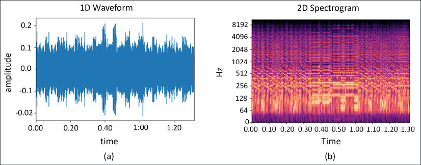
Figure 11.2: Continuous or audio domain representation of music. a) 1D waveforms are a direct representation of audio signals. b) 2D representations of audio data can be in the form of spectrograms with one axis as time and second axis as frequency
As shown in the figure, audio domain representations can be directly as 1D waveforms or 2D spectrograms:
- The 1D waveform is a direct representation of the audio signal, with the x-axis as time and the y-axis as changes to the signal
- The 2D spectrogram introduces time as the x-axis and frequency as the y-axis
We typically use Short-Time Fourier Transformation (STFT) to convert from 1D waveform to 2D spectrogram. Based on how we achieve the final spectrogram, there are different varieties such as Mel-spectrograms or magnitude spectrograms.
On the other hand, discrete or symbolic representation makes use of discrete symbols to capture information related to pitch, duration, chords, and so on. Even though less expressive than audio-domain representation, symbolic representation is widely used across different music generation works. This popularity is primarily due to the ease of understanding and handling such a representation. Figure 11.3 showcases a sample symbolic representation of a music score:

Figure 11.3: Discrete or symbolic representation of music
As shown in the figure, a symbolic representation captures information using various symbols/positions. MIDI, or Musical Instrument Digital Interface, is an interoperable format used by musicians to create, compose, perform, and share music. It is a common format used by various electronic musical instruments, computers, smartphones, and even software to read and play music files.
The symbolic representation can be designed to capture a whole lot of events such as note-on, note-off, time shift, bar, track, and so on. To understand the upcoming sections and the scope of this chapter, we will only focus on two main events, note-on and note-off. The MIDI format captures 16 channels (numbered 0 to 15), 128 notes, and 128 loudness settings (also called velocity). There are a number of other formats as well, but for the purposes of this chapter, we will leverage MIDI-based music files only as these are widely used, expressive, interoperable, and easy to understand.
To interact with, manipulate, and finally generate music, we require an interface for MIDI files. We'll make use of music21 as our library of choice for loading and processing MIDI files in Python. In the following code snippet, we load a sample MIDI file using music21. We then use its utility function to visualize the information in the file:
from music21 import converter
midi_filepath = 'Piano Sonata No.27.mid'
midi_score = converter.parse(midi_filepath).chordify()
# text-form
print(midi_score.show('text'))
# piano-roll form
print(midi_score.show())
We have covered quite some ground so far in terms of understanding the overall music generation landscape and a few important representation techniques. Next, we will get started with music generation itself.
Music generation using LSTMs
As we saw in the previous section, music is a continuous signal, which is a combination of sounds from various instruments and voices. Another characteristic is the presence of structural recurrent patterns which we pay attention to while listening. In other words, each musical piece has its own characteristic coherence, rhythm, and flow.
Such a setup is similar to the case of text generation we saw in Chapter 9, The Rise of Methods for Text Generation. In the case of text generation, we saw the power and effectiveness of LSTM-based networks. In this section, we will extend a stacked LSTM network for the task of music generation.
To keep things simple and easy to implement, we will focus on a single instrument/monophonic music generation task. Let's first look at the dataset and think about how we would prepare it for our task of music generation.
Dataset preparation
MIDI is an easy-to-use format which helps us extract a symbolic representation of music contained in the files. For the hands-on exercises in this chapter, we will make use of a subset of the massive public MIDI dataset collected and shared by reddit user u/midi_man, which is available at this link:
The subset is based on classical piano pieces by great musicians such as Beethoven, Bach, Bartok, and the like. The subset can be found in a zipped folder, midi_dataset.zip, along with the code in this book's GitHub repository.
As mentioned previously, we will make use of music21 to process the subset of this dataset and prepare our data for training the model. As music is a collection of sounds from various instruments and voices/singers, for the purpose of this exercise we will first use the chordify() function to extract chords from the songs. The following snippet helps us to get a list of MIDI scores in the required format:
from music21 import converter
data_dir = 'midi_dataset'
# list of files
midi_list = os.listdir(data_dir)
# Load and make list of stream objects
original_scores = []
for midi in tqdm(midi_list):
    score = converter.parse(os.path.join(data_dir,midi))
    original_scores.append(score)
# Merge notes into chords
original_scores = [midi.chordify() for midi in tqdm(original_scores)]
Once we have the list of scores, the next step is to extract notes and their corresponding timing information. For extracting these details, music21 has simple-to-use interfaces such as element.pitch and element.duration.
The following snippet helps us extract such information from MIDI files and prepare two parallel lists:
# Define empty lists of lists
original_chords = [[] for _ in original_scores]
original_durations = [[] for _ in original_scores]
original_keys = []
# Extract notes, chords, durations, and keys
for i, midi in tqdm(enumerate(original_scores)):
    original_keys.append(str(midi.analyze('key')))
    for element in midi:
        if isinstance(element, note.Note):
            original_chords[i].append(element.pitch)
            original_durations[i].append(element.duration.quarterLength)
        elif isinstance(element, chord.Chord):
            original_chords[i].append('.'.join(str(n) for n in element.pitches))
            original_durations[i].append(element.duration.quarterLength)
We take one additional step to reduce the dimensionality. While this is an optional step, we recommend this in order to keep the task tractable as well as to keep the model training requirements within limits. The following snippet reduces the list of notes/chords and duration to only songs in the C major key:
# Create list of chords and durations from songs in C major
major_chords = [c for (c, k) in tqdm(zip(original_chords, original_keys)) if (k == 'C major')]
major_durations = [c for (c, k) in tqdm(zip(original_durations, original_keys)) if (k == 'C major')]
Now we have pre-processed our dataset, the next step is to transform the notes/chords and duration-related information into consumable form. As we did in the case of text generation, one simple method is to create a mapping of symbols to integers. Once transformed into integers, we can use them as inputs to an embedding layer of the model, which gets fine-tuned during the training process itself. The following snippet prepares the mapping and presents a sample output as well:
def get_distinct(elements):
    # Get all pitch names
    element_names = sorted(set(elements))
    n_elements = len(element_names)
    return (element_names, n_elements)
def create_lookups(element_names):
    # create dictionary to map notes and durations to integers
    element_to_int = dict((element, number) for number, element in enumerate(element_names))
    int_to_element = dict((number, element) for number, element in enumerate(element_names))
    return (element_to_int, int_to_element)
# get the distinct sets of notes and durations
note_names, n_notes = get_distinct([n for chord in major_chords for n in chord])
duration_names, n_durations = get_distinct([d for dur in major_durations for d in dur])
distincts = [note_names, n_notes, duration_names, n_durations]
with open(os.path.join(store_folder, 'distincts'), 'wb') as f:
    pickle.dump(distincts, f)
# make the lookup dictionaries for notes and durations and save
note_to_int, int_to_note = create_lookups(note_names)
duration_to_int, int_to_duration = create_lookups(duration_names)
lookups = [note_to_int, int_to_note, duration_to_int, int_to_duration]
with open(os.path.join(store_folder, 'lookups'), 'wb') as f:
    pickle.dump(lookups, f)
print("Unique Notes={} and Duration values={}".format(n_notes,n_durations))
Unique Notes=2963 and Duration values=18
We now have the mapping ready. In the following snippet, we prepare the training dataset as sequences of length 32 with their corresponding target as the very next token in the sequence:
# Set sequence length
sequence_length = 32
# Define empty array for training data
train_chords = []
train_durations = []
target_chords = []
target_durations = []
# Construct train and target sequences for chords and durations
# hint: refer back to Chapter 9 where we prepared similar
# training data
# sequences for an LSTM-based text generation network
for s in range(len(major_chords)):
    chord_list = [note_to_int[c] for c in major_chords[s]]
    duration_list = [duration_to_int[d] for d in major_durations[s]]
    for i in range(len(chord_list) - sequence_length):
        train_chords.append(chord_list[i:i+sequence_length])
        train_durations.append(duration_list[i:i+sequence_length])
        target_chords.append(chord_list[i+1])
        target_durations.append(duration_list[i+1])
As we've seen, the dataset preparation stage was mostly straightforward apart from a few nuances associated with the handling of MIDI files. The generated sequences and their corresponding targets are shown in the following output snippet for reference:
print(train_chords[0])
array([ 935, 1773, 2070, 2788,  244,  594, 2882, 1126,  152, 2071,
        2862, 2343, 2342,  220,  221, 2124, 2123, 2832, 2584, 939,
        1818, 2608, 2462,  702,  935, 1773, 2070, 2788,  244, 594,
        2882, 1126])
print(target_chords[0])
1773
print(train_durations[0])
array([ 9,  9,  9, 12,  5,  8,  2,  9,  9,  9,  9,  5,  5,  8,  2,
        5,  5,  9,  9,  7,  3,  2,  4,  3,  9,  9,  9, 12,  5,  8,
        2,  9])
print(target_durations[0])
9
The transformed dataset is now a sequence of numbers, just like in the text generation case. The next item on the list is the model itself.
LSTM model for music generation
As mentioned earlier, our first music generation model will be an extended version of the LSTM-based text generation model from Chapter 9, The Rise of Methods for Text Generation. Yet there are a few caveats that we need to handle and necessary changes that need to be made before we can use the model for this task.
Unlike text generation (using Char-RNN) where we had only a handful of input symbols (lower- and upper-case alphabets, numbers), the number of symbols in the case of music generation is pretty large (~500). Add to this list of symbols a few additional ones required for time/duration related information as well. With this larger input symbol list, the model requires more training data and capacity to learn (capacity in terms of the number of LSTM units, embedding size, and so on).
The next obvious change we need to take care of is the model's capability to take two inputs for every timestep. In other words, the model should be able to take the notes as well as duration information as input at every timestep and generate an output note with its corresponding duration. To do so, we leverage the functional tensorflow.keras API to prepare a multi-input multi-output architecture in place.
As discussed in detail in Chapter 9, The Rise of Methods for Text Generation, stacked LSTMs have a definite advantage in terms of being able to learn more sophisticated features over networks with a single LSTM layer. In addition to that, we also discussed attention mechanisms and how they help in alleviating issues inherent to RNNs, such as difficulties in handling long-range dependencies. Since music is composed of local as well as global structures which are perceivable in the form of rhythm and coherence, attention mechanisms can certainly make an impact. The following code snippet prepares a multi-input stacked LSTM network in the manner discussed:
def create_network(n_notes, n_durations, embed_size = 100,                                          rnn_units = 256):
    """ create the structure of the neural network """
    notes_in = Input(shape = (None,))
    durations_in = Input(shape = (None,))
    x1 = Embedding(n_notes, embed_size)(notes_in)
    x2 = Embedding(n_durations, embed_size)(durations_in)
    x = Concatenate()([x1,x2])
    x = LSTM(rnn_units, return_sequences=True)(x)
    x = LSTM(rnn_units, return_sequences=True)(x)
    # attention
    e = Dense(1, activation='tanh')(x)
    e = Reshape([-1])(e)
    alpha = Activation('softmax')(e)
    alpha_repeated = Permute([2, 1])(RepeatVector(rnn_units)(alpha))
    c = Multiply()([x, alpha_repeated])
    c = Lambda(lambda xin: K.sum(xin, axis=1), output_shape=(rnn_units,))(c)


    notes_out = Dense(n_notes, activation = 'softmax', name = 'pitch')(c)
    durations_out = Dense(n_durations, activation = 'softmax', name = 'duration')(c)

    model = Model([notes_in, durations_in], [notes_out, durations_out])
    model.compile(loss=['sparse_categorical_crossentropy',
                        'sparse_categorical_crossentropy'], optimizer=RMSprop(lr = 0.001))
    return model
The model prepared using the preceding snippet is a multi-input network (one input each for notes and durations respectively). Each of the inputs is transformed into vectors using respective embedding layers. We then concatenate both inputs and pass them through a couple of LSTM layers followed by a simple attention mechanism. After this point, the model again diverges into two outputs (one for the next note and the other for the duration of that note). Readers are encouraged to use keras utilities to visualize the network on their own.
Training this model is as simple as calling the fit() function on the keras model object. We train the model for about 100 epochs. Figure 11.4 depicts the learning progress of the model across different epochs:

Figure 11.4: Model output as the training progresses across epochs
As shown in the figure, the model is able to learn a few repeating patterns and generate music. Here, we made use of temperature-based sampling as our decoding strategy. As discussed in Chapter 9, The Rise of Methods for Text Generation, readers can experiment with techniques such as greedy decoding, pure sampling-based decoding, and other such strategies to see how the output music quality changes.
This was a very simple implementation of music generation using deep learning models. We drew analogies with concepts learned in the previous two chapters on text generation. Next, let's do some music generation using adversarial networks.
Music generation using GANs
In the previous section, we tried our hand at music generation using a very simple LSTM-based model. Now, let's raise the bar a bit and try to see how we can generate music using a GAN. In this section, we will leverage the concepts related to GANs that we have learned in the previous chapters and apply them to generating music.
We've already seen that music is continuous and sequential in nature. LSTMs or RNNs in general are quite adept at handling such datasets. We have also seen that, over the years, various types of GANs have been proposed to train deep generative networks efficiently.
Combining the power of LSTMs and GAN-based generative networks, Mogren et al. presented Continuous Recurrent Neural Networks with Adversarial Training: C-RNN-GAN4 in 2016 as a method for music generation. This is a straightforward yet effective implementation for music generation. As in the previous section, we will keep things simple and focus only on monophonic music generation, even though the original paper mentions using features such as tone length, frequency, intensity, and time apart from music notes. The paper also mentions a technique called feature mapping to generate polyphonic music (using the C-RNN-GAN-3 variant). We will only focus on understanding the basic architecture and pre-processing steps and not try to implement the paper as-is. Let's begin with defining each of the components of our music-generating GAN.
Generator network
The generator network in this setup is a simple stack of multiple dense, leaky ReLU, and batch normalization layers. We start off with a random vector z of a given dimension and pass it through different non-linearities to achieve a final output of desired shape. This stack is shown in the following snippet, where we use tensorflow.keras to prepare our generator model:
def build_generator(latent_dim,seq_shape):
  model = Sequential()
  model.add(Dense(256, input_dim=latent_dim))
  model.add(LeakyReLU(alpha=0.2))
  model.add(BatchNormalization(momentum=0.8))
  model.add(Dense(512))
  model.add(LeakyReLU(alpha=0.2))
  model.add(BatchNormalization(momentum=0.8))
  model.add(Dense(1024))
  model.add(LeakyReLU(alpha=0.2))
  model.add(BatchNormalization(momentum=0.8))
  model.add(Dense(np.prod(seq_shape), activation='tanh'))
  model.add(Reshape(seq_shape))
  model.summary()
  noise = Input(shape=(latent_dim,))
  seq = model(noise)
  return Model(noise, seq)
The generator model is a fairly straightforward implementation which highlights the effectiveness of a GAN-based generative model. Next, let us prepare the discriminator model.
Discriminator network
In a GAN setup, the discriminator's job is to differentiate between real and generated (or fake) samples. In this case, since the sample to be checked is a musical piece, the model needs to have the ability to handle sequential input.
In order to handle sequential input samples, we use a simple stacked RNN network. The first recurrent layer is an LSTM layer with 512 units, followed by a bi-directional LSTM layer. The bi-directionality of the second layer helps the discriminator learn about the context better by viewing what came before and after a particular chord or note. The recurrent layers are followed by a stack of dense layers and a final sigmoid layer for the binary classification task. The discriminator network is presented in the following code snippet:
def build_discriminator(seq_shape):
  model = Sequential()
  model.add(LSTM(512, input_shape=seq_shape, return_sequences=True))
  model.add(Bidirectional(LSTM(512)))
  model.add(Dense(512))
  model.add(LeakyReLU(alpha=0.2))
  model.add(Dense(256))
  model.add(LeakyReLU(alpha=0.2))
  model.add(Dense(1, activation='sigmoid'))
  model.summary()
  seq = Input(shape=seq_shape)
  validity = model(seq)
  return Model(seq, validity)
As shown in the snippet, the discriminator is also a very simple model consisting of a few recurrent and dense layers. Next, let us combine all these components and train the overall GAN.
Training and results
The first step is to instantiate the generator and discriminator models using the utilities we presented in the previous sections. Once we have these objects, we combine the generator and discriminator into a stack to form the overall GAN. The following snippet presents the instantiation of the three networks:
rows = 100
seq_length = rows
seq_shape = (seq_length, 1)
latent_dim = 1000
optimizer = Adam(0.0002, 0.5)
# Build and compile the discriminator
discriminator = build_discriminator(seq_shape)
discriminator.compile(loss='binary_crossentropy', optimizer=optimizer, metrics=['accuracy'])
# Build the generator
generator = build_generator(latent_dim,seq_shape)
# The generator takes noise as input and generates note sequences
z = Input(shape=(latent_dim,))
generated_seq = generator(z)
# For the combined model we will only train the generator
discriminator.trainable = False
# The discriminator takes generated images as input and determines validity
validity = discriminator(generated_seq)
# The combined model  (stacked generator and discriminator)
# Trains the generator to fool the discriminator
gan = Model(z, validity)
gan.compile(loss='binary_crossentropy', optimizer=optimizer)
As we have done in the previous chapters, the discriminator training is first set to false before it is stacked into the GAN model object. This ensures that only the generator weights are updated during the generation cycle and not the discriminator weights. We prepare a custom training loop just as we have presented a number of times in previous chapters.
For the sake of completeness, we present it again here for reference:
def train(latent_dim,
          notes,
          generator,
          discriminator,
          gan,
          epochs,
          batch_size=128,
          sample_interval=50):
  disc_loss =[]
  gen_loss = []
  n_vocab = len(set(notes))
  X_train, y_train = prepare_sequences(notes, n_vocab)
  # ground truths
  real = np.ones((batch_size, 1))
  fake = np.zeros((batch_size, 1))
  for epoch in range(epochs):
      idx = np.random.randint(0, X_train.shape[0], batch_size)
      real_seqs = X_train[idx]
      noise = np.random.normal(0, 1, (batch_size, latent_dim))
      # generate a batch of new note sequences
      gen_seqs = generator.predict(noise)
      # train the discriminator
      d_loss_real = discriminator.train_on_batch(real_seqs, real)
      d_loss_fake = discriminator.train_on_batch(gen_seqs, fake)
      d_loss = 0.5 * np.add(d_loss_real, d_loss_fake)
      #  train the Generator
      noise = np.random.normal(0, 1, (batch_size, latent_dim))
      g_loss = gan.train_on_batch(noise, real)
      # visualize progress
      if epoch % sample_interval == 0:
        print ("%d [D loss: %f, acc.: %.2f%%] [G loss: %f]" % (epoch, d_loss[0],100*d_loss[1],g_loss))
        disc_loss.append(d_loss[0])
        gen_loss.append(g_loss)
  generate(latent_dim, generator, notes)
  plot_loss(disc_loss,gen_loss)
We have used the same training dataset as in the previous section. We train our setup for about 200 epochs with a batch size of 64. Figure 11.5 is a depiction of discriminator and generator losses over training cycles, along with a few outputs at different intervals:

Figure 11.5: a) Discriminator and generator losses as the training progresses over time. b) The output from the generator model at different training intervals
The outputs shown in the figure highlight the potential of a GAN-based music generation setup. Readers may choose to experiment with different datasets or even the details mentioned in the C-RNN-GAN paper by Mogren et al. The generated MIDI files can be played using the MuseScore app.
The output from this GAN-based model as compared to the LSTM-based model from the previous section might feel a bit more refined (though this is purely subjective given our small datasets). This could be attributed to GANs' inherent ability to better model the generation process compared to an LSTM-based model. Please refer to Chapter 6, Image Generation with GANs, for more details on the topology of generative models and their respective strengths.
Now that we have seen two variations of monophonic music generation, let us graduate toward polyphonic music generation using MuseGAN.
MuseGAN – polyphonic music generation
The two models we have trained so far have been simplified versions of how music is actually perceived. While limited, both the attention-based LSTM model and the C-RNN-GAN based model helped us to understand the music generation process very well. In this section, we will build on what we've learned so far and make a move toward preparing a setup which is as close to the actual task of music generation as possible.
In 2017, Dong et al. presented a GAN-type framework for multi-track music generation in their work titled MuseGAN: Multi-track Sequential Generative Adversarial Networks for Symbolic Music Generation and Accompaniment.5 The paper is a detailed explanation of various music-related concepts and how Dong and team tackled them. To keep things within the scope of this chapter and without losing details, we will touch upon the important contributions of the work and then proceed toward the implementation. Before we get onto the "how" part, let's understand the three main properties related to music that the MuseGAN work tries to take into account:
- Multi-track interdependency: As we know, most songs that we listen to are usually composed of multiple instruments such as drums, guitars, bass, vocals, and so on. There is a high level of interdependency in how these components play out for the end-user/listener to perceive coherence and rhythm.
- Musical texture: Musical notes are often grouped into chords and melodies. These groupings are characterized by a high degree of overlap and not necessarily chronological ordering (this simplification of chronological ordering is usually applied in most known works associated with music generation). The chronological ordering comes not only as part of the need for simplification but also as a generalization from the NLP domain, language generation in particular.
- Temporal structure: Music has a hierarchical structure where a song can be seen as being composed of paragraphs (at the highest level). A paragraph is composed of various phrases, which are in turn composed of multiple bars, and so on. Figure 11.6 depicts this hierarchy pictorially:

Figure 11.6: Temporal structure of a song
- As shown in the figure, a bar is further composed of beats and at the lowest level, we have pixels. The authors of MuseGAN mention a bar as the compositional unit, as opposed to notes, which we have been considering the basic unit so far. This is done in order to account for grouping of notes from the multi-track setup.
MuseGAN works toward solving these three major challenges through a unique framework based on three music generation approaches. These three basic approaches make use of jamming, hybrid, and composer models. We will briefly explain these now.
Jamming model
If we were to extrapolate the simplified-monophonic GAN setup from the previous section to a polyphonic setup, the simplest method would be to make use of multiple generator-discriminator combinations, one for each instrument. The jamming model is precisely this setup, where M multiple independent generators prepare music from their respective random vectors. Each generator has its own critic/discriminator, which helps in training the overall GAN. This setup is depicted in Figure 11.7:

Figure 11.7: Jamming model composed of M generator and discriminator pairs for generating multi-track outputs
As shown in the preceding figure, the jamming setup imitates a grouping of musicians who create music by improvising independently and without any predefined arrangement.
Composer model
As the name suggests, this setup assumes that the generator is a typical human composer capable of creating multi-track piano rolls, as shown in Figure 11.8:

Figure 11.8: Composer model composed of a single generator capable of generating M tracks and a single discriminator for detecting fake versus real samples
As shown in the figure, the setup only has a single discriminator to detect real or fake (generated) samples. This model requires only one common random vector z as opposed to M random vectors in the previous jamming model setup.
Hybrid model
This is an interesting take that arises by combining the jamming and composer models. The hybrid model has M independent generators that make use of their respective random vectors, which are also called intra-track random vectors. Each generator also takes an additional random vector called the inter-track random vector. This additional vector is supposed to imitate the composer and help in the coordination of the independent generators. Figure 11.9 depicts the hybrid model, with M generators each taking intra-track and inter-track random vectors as input:

Figure 11.9: Hybrid model composed of M generators and a single discriminator. Each generator takes two inputs in the form of inter-track and intra-track random vectors
As shown in the figure, the hybrid model with its M generators works with only a single discriminator to predict whether a sample is real or fake. The advantage of combining both jamming and composer models is in terms of flexibility and control at the generator end. Since we have M different generators, the setup allows for flexibility to choose different architectures (different input sizes, filters, layers, and so on) for different tracks, as well as additional control via the inter-track random vector to manage coordination amongst them.
Apart from these three variants, the authors of MuseGAN also present a temporal model, which we discuss next.
Temporal model
The temporal structure of music was one of the three aspects we discussed as top priorities for the MuseGAN setup. The three variants explained in the previous sections, jamming, composer, and hybrid models, all work at the bar level. In other words, each of these models generates multi-track music bar by bar, but possibly with no coherence or continuity between two successive bars. This is different from the hierarchical structure where a group of bars makes up a phrase, and so on.
To maintain coherence and the temporal structure of the song being generated, the authors of MuseGAN present a temporal model. While generating from scratch (as one of the modes), this additional model helps in generating fixed-length phrases by taking bar-progression as an additional dimension. This model consists of two sub-components, the temporal structure generator Gtemp and the bar generator Gbar. This setup is presented in Figure 11.10:

Figure 11.10: Temporal model with its two sub-components, temporal structure generator Gtemp and bar generator Gbar
The temporal structure generator maps a noise vector z to a sequence of latent vectors ![]() . This latent vector
. This latent vector ![]() carries temporal information and is then used by Gbar to generate music bar by bar. The overall setup for the temporal model is formulated as follows:
carries temporal information and is then used by Gbar to generate music bar by bar. The overall setup for the temporal model is formulated as follows:

The authors note that this setup is similar to some of the works on video generation, and cite references for further details. The authors also mention another setting where a conditional setup is presented for the generation of temporal structure by learning from a human-generated track sequence.
We have covered details on the specific building blocks for the MuseGAN setup. Let's now dive into how these components make up the overall system.
MuseGAN
The overall MuseGAN setup is a complex architecture composed of a number of moving parts. To bring things into perspective, the paper presents experiments with jamming, composer, and hybrid generation approaches at a very high level. To ensure temporal structure, the setup makes use of the two-step temporal model approach we discussed in the previous section. A simplified version of the MuseGAN architecture is presented in Figure 11.11:

Figure 11.11: Simplified MuseGAN architecture consisting of a hybrid model with M generators and a single discriminator, along with a two-stage temporal model for generating phrase coherent output
As shown in the figure, the setup makes use of a temporal model for certain tracks and direct random vectors for others. The outputs from temporal models, as well as direct inputs, are then concatenated (or summed) before they are passed to the bar generator model.
The bar generator then creates music bar by bar and is evaluated using a critic or discriminator model. In the coming section, we will briefly touch upon implementation details for both the generator and critic models.
Please note that the implementation presented in this section is close to the original work but not an exact replication. We have taken certain shortcuts in order to simplify and ease the understanding of the overall architecture. Interested readers may refer to official implementation details and the code repository mentioned in the cited work.
Generators
As mentioned in the previous section, the generator setup depends on whether we are using the jamming, composer, or hybrid approach. For simplicity, we will focus only on the hybrid setup where we have multiple generators, one for each track.
One set of generators focuses on tracks which require temporal coherence; for instance, components such as melody are long sequences (more than one bar long) and coherence between them is an important factor. For such tracks, we use a temporal architecture as shown in the following snippet:
def build_temporal_network(z_dim, n_bars, weight_init):
    input_layer = Input(shape=(z_dim,), name='temporal_input')
    x = Reshape([1, 1, z_dim])(input_layer)
    x = Conv2DTranspose(
        filters=512,
        kernel_size=(2, 1),
        padding='valid',
        strides=(1, 1),
        kernel_initializer=weight_init
    )(x)
    x = BatchNormalization(momentum=0.9)(x)
    x = Activation('relu')(x)
    x = Conv2DTranspose(
        filters=z_dim,
        kernel_size=(n_bars - 1, 1),
        padding='valid',
        strides=(1, 1),
        kernel_initializer=weight_init
    )(x)
    x = BatchNormalization(momentum=0.9)(x)
    x = Activation('relu')(x)
    output_layer = Reshape([n_bars, z_dim])(x)
    return Model(input_layer, output_layer)
As shown, the temporal model firstly reshapes the random vector to desired dimensions, then passes it through transposed convolutional layers to expand the output vector so that it spans the length of specified bars.
For the tracks where we do not require inter-bar coherence, we directly use the random vector z as-is. Groove or beat-related information covers such tracks in practice.
The outputs from the temporal generator and the direct random vectors are first concatenated to prepare a larger coordinated vector. This vector then acts as an input to the bar generator Gbar shown in the following snippet:
def build_bar_generator(z_dim, n_steps_per_bar, n_pitches, weight_init):
    input_layer = Input(shape=(z_dim * 4,), name='bar_generator_input')
    x = Dense(1024)(input_layer)
    x = BatchNormalization(momentum=0.9)(x)
    x = Activation('relu')(x)
    x = Reshape([2, 1, 512])(x)
    x = Conv2DTranspose(
        filters=512,
        kernel_size=(2, 1),
        padding='same',
        strides=(2, 1),
        kernel_initializer=weight_init
    )(x)
    x = BatchNormalization(momentum=0.9)(x)
    x = Activation('relu')(x)
    x = Conv2DTranspose(
        filters=256,
        kernel_size=(2, 1),
        padding='same',
        strides=(2, 1),
        kernel_initializer=weight_init
    )(x)
    x = BatchNormalization(momentum=0.9)(x)
    x = Activation('relu')(x)
    x = Conv2DTranspose(
        filters=256,
        kernel_size=(2, 1),
        padding='same',
        strides=(2, 1),
        kernel_initializer=weight_init
    )(x)
    x = BatchNormalization(momentum=0.9)(x)
    x = Activation('relu')(x)
    x = Conv2DTranspose(
        filters=256,
        kernel_size=(1, 7),
        padding='same',
        strides=(1, 7),
        kernel_initializer=weight_init
    )(x)
    x = BatchNormalization(momentum=0.9)(x)
    x = Activation('relu')(x)
    x = Conv2DTranspose(
        filters=1,
        kernel_size=(1, 12),
        padding='same',
        strides=(1, 12),
        kernel_initializer=weight_init
    )(x)
    x = Activation('tanh')(x)
    output_layer = Reshape([1, n_steps_per_bar, n_pitches, 1])(x)
    return Model(input_layer, output_layer)
The snippet shows that the bar generator consists of a dense layer followed by batch-normalization, before a stack of transposed convolutional layers, which help to expand the vector along time and pitch dimensions.
Critic
The critic model is simpler compared to the generator we built in the previous section. The critic is basically a convolutional WGAN-GP model (similar to WGAN, covered in Chapter 6, Image Generation with GANs), which takes the output from the bar generator, as well as real samples, to detect whether the generator output is fake or real. The following snippet presents the critic model:
def build_critic(input_dim, weight_init, n_bars):
    critic_input = Input(shape=input_dim, name='critic_input')
    x = critic_input
    x = conv_3d(x,
                num_filters=128,
                kernel_size=(2, 1, 1),
                stride=(1, 1, 1),
                padding='valid',
                weight_init=weight_init)
    x = conv_3d(x,
                num_filters=64,
                kernel_size=(n_bars - 1, 1, 1),
                stride=(1, 1, 1),
                padding='valid',
                weight_init=weight_init)
    x = conv_3d(x,
                num_filters=64,
                kernel_size=(1, 1, 12),
                stride=(1, 1, 12),
                padding='same',
                weight_init=weight_init)
    x = conv_3d(x,
                num_filters=64,
                kernel_size=(1, 1, 7),
                stride=(1, 1, 7),
                padding='same',
                weight_init=weight_init)
    x = conv_3d(x,
                num_filters=64,
                kernel_size=(1, 2, 1),
                stride=(1, 2, 1),
                padding='same',
                weight_init=weight_init)
    x = conv_3d(x,
                num_filters=64,
                kernel_size=(1, 2, 1),
                stride=(1, 2, 1),
                padding='same',
                weight_init=weight_init)
    x = conv_3d(x,
                num_filters=128,
                kernel_size=(1, 4, 1),
                stride=(1, 2, 1),
                padding='same',
                weight_init=weight_init)
    x = conv_3d(x,
                num_filters=256,
                kernel_size=(1, 3, 1),
                stride=(1, 2, 1),
                padding='same',
                weight_init=weight_init)
    x = Flatten()(x)
    x = Dense(512, kernel_initializer=weight_init)(x)
    x = LeakyReLU()(x)
    critic_output = Dense(1,
                          activation=None,
                          kernel_initializer=weight_init)(x)
    critic = Model(critic_input, critic_output)
    return critic
One major point to note here is the use of 3D convolutional layers. We typically make use of 2D convolutions for a majority of tasks. In this case, since we have 4-dimensional inputs, a 3D convolutional layer is required for handling the data correctly.
We use these utilities to prepare 4 different generators, one for each track, into a common generator model object. In the next step, we prepare the training setup and generate some sample music.
Training and results
We have all the components ready. The final step is to combine them and train in the manner a typical WGAN-GP is trained. The authors of the paper mention that the model achieves stable performance if they update the generators once for every 5 updates of the discriminator. We follow a similar setup to achieve the results shown in Figure 11.12:

Figure 11.12: Results from MuseGAN setup showcase multi-track output, which seems to be coherent across bars and has a consistent rhythm to it
As shown in the figure, the multi-track polyphonic output from MuseGAN indeed seems quite impressive. We urge readers to use a MIDI player (or even MuseScore itself) to play the generated music samples in order to understand the complexity of the output, along with the improvement over the simpler models prepared in the earlier sections of the chapter.
Summary
Congratulations on completing yet another complex chapter. In this chapter, we covered quite a bit of ground in terms of building an understanding of music as a source of data, and then various methods of generating music using generative models.
In the first section of this chapter, we briefly discussed the two components of music generation, namely score and performance generation. We also touched upon different use cases associated with music generation. The next section focused on different methods for music representation. At a high level, we discussed continuous and discrete representation techniques. We primarily focused on 1D waveforms and 2D spectrograms as main representations in the audio or continuous domain. For symbolic or discrete representation, we discussed notes/chords-based sheet music. We also performed a quick hands-on exercise using the music21 library to transform a given MIDI file into readable sheet music.
Once we had some basic understanding of how music can be represented, we turned toward building music generation models. The first and the simplest method we worked upon was based on a stacked LSTM architecture. The model made use of an attention mechanism and symbolic representation to generate the next set of notes. This LSTM-based model helped us to get a peek into the music generation process.
The next section focused on using a GAN setup to generate music. We designed our GAN similar to C-RNN-GAN presented by Mogren et al. The results were very encouraging and gave us a good insight into how an adversarial network can be used for the task of music generation.
During the first two hands-on exercises, we limited our music generation process to only monophonic music to keep things simple. In the final section of this chapter, our aim was to understand the complexities and techniques required to generate polyphonic/multi-track music. We discussed in detail MuseGAN, a polyphonic/multi-track GAN-based music generation architecture presented by Dong et al. in 2017. Dong and team discussed multi-track interdependency, musical texture, and temporal structure as three main aspects that should be handled by any multi-track music generation model. They presented three variants for music generation in the form of jamming, composer, and hybrid models. They also presented a discussion on temporal and bar generation models to bring things into perspective. The MuseGAN paper presents MuseGAN as a complex combination of these smaller components/models to handle multi-track/polyphonic music generation. We leveraged this understanding to build a simplified version of this work and generate polyphonic music of our own.
This chapter provided us with a look into yet another domain which can be handled using generative models. In the next chapter, we will level things up and focus on the exciting field of reinforcement learning. Using RL, we will build some cool applications as well. Stay tuned.
References
- Butcher, M. (2019, July 23). It looks like TikTok has acquired Jukedeck, a pioneering music AI UK startup. TechCrunch. https://techcrunch.com/2019/07/23/it-looks-like-titok-has-acquired-jukedeck-a-pioneering-music-ai-uk-startup/
- Apple. (2021). GarageBand for Mac - Apple. https://www.apple.com/mac/garageband/
- Magenta. (n.d.) Make Music and Art Using Machine Learning. https://magenta.tensorflow.org/
- Mogren, O. (2016). C-RNN-GAN: Continuous recurrent neural networks with adversarial training. Constructive Machine Learning Workshop (CML) at NIPS 2016 in Barcelona, Spain, December 10. https://arxiv.org/abs/1611.09904
- Dong, H-W., Hsiao, W-Y., Yang, L-C., & Yang, Y-H. (2017). MuseGAN: Multi-Track Sequential Generative Adversarial Networks for Symbolic Music Generation and Accompaniment. The Thirty-Second AAAI Conference on Artificial Intelligence (AAAI-18). https://salu133445.github.io/musegan/pdf/musegan-aaai2018-paper.pdf